Gross is fiction. Trade net.
Costs are among the assumptions most likely to be underestimated in research and to deteriorate live or with scale. This guide covers the whole chain: where costs come from, how the engine books them in each execution mode, the turnover arithmetic that converts basis points into Sharpe decay, and the rebalancing-policy layer that is your first and cheapest cost control. Every number is measured on the engine — including two traps we demonstrate on real data rather than warn about abstractly.
The gross backtest is a fiction
Every gross equity curve describes a strategy nobody can trade. The only honest question is how far from tradeable it is.
Here is the scale of the gap, measured. A 126-day cross-sectional momentum strategy — top 3 of 8 multi-asset ETFs, monthly rebalance, 2007–2026 — earns a 10.89% CAGR gross. The same strategy, same signal, same dates, at 50 bps per side pays $121,778 in cumulative costs against $100,000 of starting capital and keeps a 7.84% CAGR. Nothing about the strategy changed. Only the price of expressing it did — and the lower capital path compounds into a $293,004 gap in final wealth.
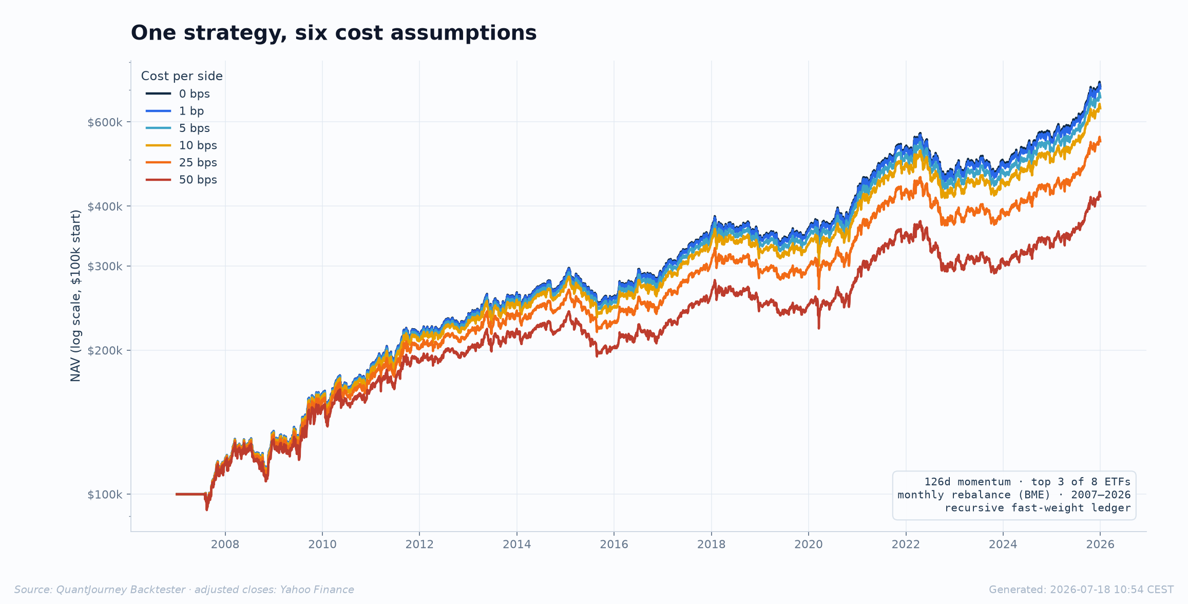
FixedBpsWeightCostModel(total_bps=…). Adjusted-close data were
refreshed from Yahoo Finance on 18 July 2026.
Costs arrive through four channels, and a realistic backtest needs a position on each. Commission — the broker's explicit fee; smallest, easiest, often near zero for institutions. Spread — you buy at the ask and sell at the bid; unavoidable, but it varies by venue, liquidity, time of day and stress regime. A flat estimate is only a first-order approximation for liquid names. Impact — your own order moves the price; grows with participation, dominates at size. And the one that never appears on a statement: the cost of not trading — every trade you suppress to save the first three leaves the portfolio drifted away from the signal that justified it. The first three channels are why turnover is expensive; the fourth is why zero turnover is not the answer. This guide measures both directions.
How the engine books a cost
Weight-mode strategies never submit orders — but a rebalance still implies trades, and implied trades cost real money. The accounting deserves to be explicit.
On each rebalance date the engine converts target weights into implied share deltas: the shares you would need to hold so that each position's value matches its target weight at today's NAV and today's price, minus the shares you already held:
The traded notional is the absolute delta times the price, and a linear cost books a constant number of basis points on every dollar of it, buys and sells alike:
The important detail is that NAV+ is the post-cost capital that also scales the reported positions.
Because the cost depends on the quantities and the quantities depend on that same NAV, the fast path solves the
fixed point below on every complete capital trajectory — it does not calculate costs from a separate gross path:
from backtester.portfolio.weight_cost import FixedBpsWeightCostModel

strategy = MyStrategy(
    ...,
    execution_mode="weights",              # fast weight accounting
    weight_cost_model=FixedBpsWeightCostModel(
        total_bps=5.0,                     # 5 bps of each implied trade's value
        min_trade_value=0.0,               # optional cost-materiality filter
    ),
)

# Default if you pass nothing: 1 bp. The engine NEVER runs weight-mode
# accounting at zero cost unless you explicitly ask for total_bps=0.
Four details in the engine's implementation are the difference between accounting and wishful thinking. One capital path: post-cost NAV, positions, quantity deltas and cost notionals reconcile to the same recursive ledger. No trading on missing marks: a bar with no price is not a tradeable bar — implied quantities persist through data gaps and no phantom "re-entry" cost appears when data resumes. Absolute-value marks: legally negative prices (futures, April 2020) cannot produce a negative trade value — costs are never a credit. Costs are outputs, not adjustments: the per-bar, per-instrument breakdown is a first-class result you can audit, aggregate and chart:
# Every run's costs are first-class outputs, not footnotes:

pdta = strategy.portfolio_data
pdta.total_transaction_costs      # $ per bar, Series
pdta.total_transaction_costs.sum()

# Weight mode: the full implied-trade audit trail
breakdown = strategy._weight_cost_breakdown
breakdown.quantity_deltas         # implied share deltas per bar
breakdown.trade_values            # |delta| x price, the traded notional
breakdown.transaction_costs       # per instrument, per bar
breakdown.total_cost_pct          # cost as fraction of NAV per bar

# Annual turnover from the same accounting that booked the costs:
traded = breakdown.trade_values.sum(axis=1)
to_ann = (traded / pdta.net_asset_value).mean() * 252
Turnover: your exposure to costs
Basis points are the price; turnover is the quantity. Cost drag is their product, and it obeys arithmetic you can do on a napkin.
Define annual turnover as traded notional over NAV, annualized — a strategy that replaces its entire book five times a year has TO ≈ 5×:
A linear cost of c basis points per side then drags returns by c·TO per year, and — since costs subtract from the mean while barely touching the volatility — lowers the Sharpe ratio proportionally:
Plug in the momentum strategy from the ladder:
Five basis points on a 5.58× strategy predicts 28 bps of return drag and about 0.02 of Sharpe per year. The same five bps on a 30.3× strategy (the daily-rebalanced variant below) produces 1.62% of measured CAGR drag — a fee war against yourself. The linear model also gives you a breakeven: the cost level at which the gross Sharpe reaches zero,
200 bps of first-order headroom sounds comfortable — but the breakeven is the wrong bar. The strategy has to beat its alternatives net, not zero, and it has to survive cost estimates being wrong by 2× in the bad direction. Which is why the ladder, not the formula, is the deliverable.
The cost ladder, measured
Six engine runs answer the question every strategy owner should be able to answer cold: what happens to my numbers per basis point?
from backtester.portfolio.weight_cost import FixedBpsWeightCostModel

results = {}
for bps in [0, 1, 5, 10, 25, 50]:
    s = XSMomentum(
        ...,                                   # identical config otherwise
        weight_cost_model=FixedBpsWeightCostModel(total_bps=bps),
    )
    await s.run_strategy()
    nav = s.portfolio_data.net_asset_value
    costs = s.portfolio_data.total_transaction_costs
    results[bps] = (nav.iloc[-1], costs.sum())

# Six engine runs, one afternoon question answered for good:
# "at what cost level does this strategy stop being worth trading?"| Cost per side | CAGR | Net Sharpe | Max DD | Total costs | Measured drag/yr | c·TO prediction |
|---|---|---|---|---|---|---|
| 0 bps | 10.89% | 0.879 | −20.1% | $0 | — | — |
| 1 bp | 10.83% | 0.875 | −20.1% | $3,321 | 0.062% | 0.056% |
| 5 bps | 10.58% | 0.857 | −20.2% | $16,180 | 0.309% | 0.279% |
| 10 bps | 10.27% | 0.835 | −20.3% | $31,328 | 0.616% | 0.558% |
| 25 bps | 9.36% | 0.768 | −20.7% | $71,155 | 1.535% | 1.395% |
| 50 bps | 7.84% | 0.656 | −22.2% | $121,778 | 3.051% | 2.790% |
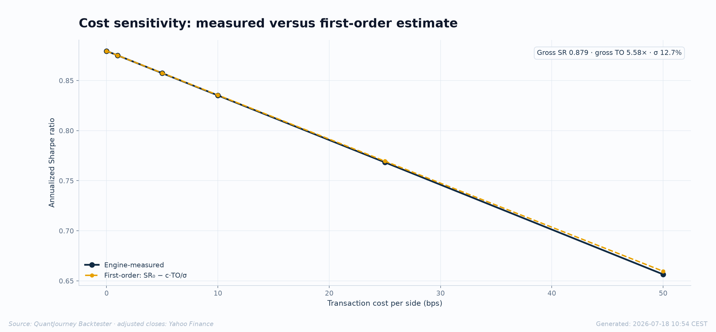
Two readings are worth taking away. First, the agreement is a useful first-order sanity check, not proof of the accounting; the stronger check is the regression identity that position changes equal costed quantity deltas and that pre-cost NAV minus booked dollars equals post-cost NAV. Second, drawdown barely moves at ordinary cost levels while Sharpe decays steadily. A 5-bps assumption produces 31 bps of measured annual CAGR drag and compounds into a $36,728 gap between the gross and net final NAVs.
Rebalancing policy is the first cost control
Before optimizing a single signal parameter, you control turnover through one declarative object: when do targets become trades?
The engine's RebalancePolicy layers five triggers, each answering a different "should we trade
today?" — a calendar schedule, a drift band on held-versus-target weights, a tracking-error trigger against a
benchmark, a signal-change trigger, a drawdown circuit breaker, and a rolling turnover budget that gates all of
them. Between rebalance dates, positions drift with prices; the engine tracks the drifted weights and trades only
when a trigger fires:
from backtester.portfolio.rebalance import RebalancePolicy

POLICIES = {
    "daily":     RebalancePolicy(frequency="D"),
    "weekly":    RebalancePolicy(frequency="W", weekday=4),
    "monthly":   RebalancePolicy(frequency="BME"),
    "m_drift":   RebalancePolicy(frequency="BME", drift_threshold=0.05),
    "m_partial": RebalancePolicy(frequency="BME", drift_threshold=0.05,
                                 partial_rebalance=True),
    "q_te_gate": RebalancePolicy(frequency="BQE",
                                 tracking_error_threshold=0.06,
                                 tracking_error_window=63,
                                 max_annual_turnover=4.0),
}

# Presets for the common cases ship with the engine:
from backtester.portfolio.rebalance import RebalancePresets
RebalancePresets.MONTHLY              # BME
RebalancePresets.MONTHLY_WITH_DRIFT   # BME + 5% drift band
RebalancePresets.RISK_MANAGED         # BME + drift + DD breaker + TO budget 4x
Same momentum strategy, 5 bps per side, six policies — six full engine runs:
| Policy | Net Sharpe | CAGR | Turnover | Rebalances | Costs paid | Drag/yr |
|---|---|---|---|---|---|---|
| Daily | 0.559 | 6.52% | 30.3× | 4,780 | $55,892 | 1.62% |
| Weekly (Fri) | 0.614 | 7.30% | 12.9× | 992 | $26,565 | 0.69% |
| Monthly (BME) | 0.857 | 10.58% | 5.58× | 229 | $16,180 | 0.31% |
| Monthly + 5% drift band | 0.556 | 6.47% | 29.4× | 1,007 | $54,005 | 1.58% |
| Monthly + drift, partial | 0.553 | 6.47% | 29.0× | 1,301 | $52,526 | 1.55% |
| Quarterly + TE 6% + TO budget 4× | 0.519 | 6.84% | 3.35× | 1,108 | $4,553 | 0.18% |
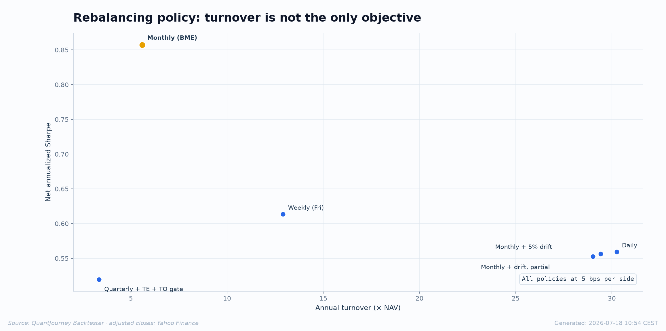
Monthly wins on this strategy — and why it wins matters more than that it wins: a 126-day momentum signal changes its mind slowly, so daily re-alignment buys mostly noise, at 30× turnover. But the table's two shock results are the real payload of this section.
Adding a 5% drift band to the monthly policy was supposed to add a safety valve. It increased turnover more than fivefold (5.58× → 29.4×) and gave back 0.30 of Sharpe. The mechanism: the engine measures drift as the gap between held weights and today's target — and this strategy recomputes its target daily, so the gap breaches the band whenever the signal moves, not just when prices drift. A drift band is a brake on a slow-target portfolio (a 60/40, a static basket) and an accelerator on a fast-signal one. Check your signal's cadence before wiring the band.
The gated policy is the cheapest in the table — 0.18% drag — and the worst investment in it: Sharpe 0.519 and a −41.9% max drawdown. The 4× rolling budget was spent by the time the GFC demanded rotation, so the strategy was forced to hold its stale winners all the way down. A momentum strategy's turnover is its risk management; a budget below its natural rate (5.58×) doesn't make it cheaper, it makes it a different strategy. Size cost gates from the strategy's measured turnover distribution — never from a round number that sounds prudent.
The general lesson from both traps: rebalancing policy is not a bolt-on cost dial. It interacts with the signal's information half-life, and the only way to see the interaction is to measure the grid — six runs, identical everything, one policy object changed at a time.
Slippage and commission, past the flat assumption
A flat bps number is the right starting model for liquid daily strategies. Three situations outgrow it — and each has a dedicated model in the engine.
In order-level execution the engine separates the two cost channels properly. Slippage adjusts the fill price itself — you buy above and sell below the theoretical mark:
When liquidity varies, a constant half-spread misprices exactly the days that hurt: spreads widen when volatility spikes. For an opening fill, the volatility-proportional model scales the spread with the previous completed bar's range — the current day's high, low and close do not exist yet,
and when your size is a nontrivial share of the day's volume, cost stops being linear at all — the Almgren-style square-root law charges for participation:
from backtester.execution import (
    FixedBpsSlippage, VolatilitySlippage, MarketImpactSlippage,
    PerShareCommission, FixedBpsCommission, TieredCommission,
)

# Constant half-spread: a first-order estimate for liquid daily ETFs
slip = FixedBpsSlippage(bps=5.0)

# Range-sensitive spread: the fill engine supplies only observable data
slip = VolatilitySlippage(vol_factor=0.1)      # spread = P * 0.1 * (H-L)/C
# At open: previous completed bar's H/L/C. At close: current completed bar.

# Almgren-style square-root impact: when YOUR size moves the price
slip = MarketImpactSlippage(
    sigma_daily=0.02,       # daily vol of the instrument
    adv=1_000_000,          # average daily volume, shares
    eta=0.1,                # temporary impact coefficient
)

# Commission schemes are orthogonal to slippage:
comm = PerShareCommission(cost_per_share=0.005, min_per_order=1.0,
                          max_pct=0.005)          # IB-style US equities
comm = FixedBpsCommission(bps=1.0)                # percent-of-notional
comm = TieredCommission(tiers=[(300, 0.0035), (3_000, 0.002),
                               (20_000, 0.0015)]) # volume-tiered
Rules of thumb for choosing: flat bps for daily-rebalanced ETFs and large-cap equities at research size;
volatility-proportional when the universe includes illiquid names or the strategy concentrates its trading in
stress regimes (mean-reversion buys crashes — its fills are systematically worse than average);
square-root impact when a live allocation is on the table and participation might exceed a few percent of ADV —
pair it with max_volume_participation. At the open, capacity is estimated from a lagged ADV window
times expected_open_volume_fraction; the simulator never borrows the completed current day's volume.
Which cost knob lives in which mode
The engine has three execution paths, and each books costs through a different door. Configuring the wrong knob is a silent no-op — so the engine warns loudly instead.
| Mode | What executes | Costs come from | Ignored (with a warning) |
|---|---|---|---|
weights + fast | Recursive post-cost weight accounting, close-to-close | weight_cost_model on implied trades | slippage_model, commission_scheme, fill_at |
weights + orders | Targets routed through real orders and fills | slippage_model + commission_scheme per fill | weight_cost_model |
orders | Explicit order objects (market, limit, stop, bracket, OCO) | slippage_model + commission_scheme per fill | weight_cost_model, rebalance_policy |
strategy = TrendBasket(
    ...,
    execution_mode="weights",
    weight_execution="orders",          # targets become real orders + fills
    slippage_model=VolatilitySlippage(vol_factor=0.1),
    commission_scheme=PerShareCommission(cost_per_share=0.005),
    fill_at="open",                     # decide on close t, fill at open t+1
    max_volume_participation=0.05,      # 5% of forecast opening capacity
    volume_lookback=20,                 # lagged ADV; never today's full volume
    expected_open_volume_fraction=0.10, # forecast 10% of ADV available at open
    rebalance_policy=RebalancePolicy(frequency="BME"),
)

# Same strategy code, heavier execution physics: integer share
# quantities, margin and buying-power checks, per-fill commission
# and slippage in the blotter - and a Transaction Cost Analysis
# chart in the report.
The fast path prices trades at the close that defined them; the orders path fills at the next open by default — decide on tonight's close, transact at tomorrow's open, with integer shares, margin checks and per-fill cost records in the blotter. Opening fills use the prior completed range for volatility slippage and lagged volume for capacity; they never read tomorrow's completed H/L/C/volume. For liquid daily strategies the two paths can agree closely, and the fast path's speed makes it the right tool for research iteration and permutation testing. Graduate to the orders path when the contract matters (integer futures, FX lots), when fill timing is part of the strategy, or as the final pre-deployment check that weight-mode results survive execution friction. If the two paths disagree materially, that gap is itself a finding: the strategy's edge lives uncomfortably close to the market's microstructure.
The cost checklist
Six habits that make every number you quote a net number.
Measure turnover before anything else
TO_ann from the engine's own trade accounting — it is the multiplier on every cost error you will ever make.
Run the ladder before tuning
Six runs, 0–50 bps. If the strategy dies below 2× your realistic cost estimate, stop here — no parameter search can outrun the drag.
Choose the rebalance policy by the signal's cadence
Slow signal, calendar policy. Fast target, no drift bands. Never gate turnover below the strategy's measured natural rate.
Match the slippage model to the liquidity regime
Flat bps → vol-proportional → square-root impact, as size and illiquidity grow. Cap participation so the simulator refuses impossible fills.
Compare variants net, always
Costs change rankings, not just levels — a faster variant can win gross and lose net. Identical cost model on every side of every comparison.
Archive the cost assumption with the run
The cost model and its parameters are part of the experiment's identity — they live in the run archive next to the seed and the data fingerprint.
We do independent validation engagements — permutation tests, walk-forward, Deflated Sharpe and rank stability on your code or track record, delivered as a signed, reproducible report.
References
- Almgren, R. & Chriss, N. (2001). Optimal Execution of Portfolio Transactions. Journal of Risk 3(2) — the impact model family behind the square-root law.
- Perold, A. F. (1988). The Implementation Shortfall: Paper Versus Reality. Journal of Portfolio Management 14(3) — why gross backtests overstate by construction.
- Grinold, R. C. & Kahn, R. N. (2000). Active Portfolio Management, ch. 16 — transaction costs, turnover and the value of trading slowly.
- Frazzini, A., Israel, R. & Moskowitz, T. (2018). Trading Costs. AQR working paper — measured institutional cost curves across 21 markets.
- Garleanu, N. & Pedersen, L. H. (2013). Dynamic Trading with Predictable Returns and Transaction Costs. Journal of Finance 68(6) — trading partially toward a moving aim portfolio.