Does your alpha predict?
A strategy is a signal plus sizing plus execution. Before any of that, one question decides whether the whole edifice can stand: does the signal actually forecast returns? The information coefficient answers it directly — the correlation between what a signal said and what the market did next. This guide computes IC, Rank IC, ICIR, lead-IC decay and permutation importance on the engine's eight-ETF universe. One of four textbook signals has a raw i.i.d. p-value below 0.05, but none clears a family-wise 5% threshold after Holm correction. That gap — between a promising estimate and evidence robust enough to deploy — is where most strategies quietly die.
The information coefficient: skill in one number
A signal ranks names; the market ranks them too, after the fact. The information coefficient is how well the two rankings agree — computed fresh every period, across the cross-section.
Formally, on each date you take the signal's value across all instruments and correlate it with each instrument's next-period return. That single number is the date's IC:
Two details matter before interpreting it. Shifting the return aligns the target correctly, but does not by itself make the signal point-in-time — every signal input must still have been available on that date. And Pearson IC is invariant to affine rescaling of the signal, not to arbitrary monotone transformations or replacing values with ranks. The rank version (Spearman) depends only on ordering, making it robust to outliers and invariant to monotone transformations of the signal:
import numpy as np
import pandas as pd
from scipy import stats

def cross_sectional_ic(signal: pd.DataFrame, fwd_return: pd.DataFrame,
                       rank: bool = False) -> pd.Series:
    """One IC per date: correlate this date's signal across names
    against each name's *next-period* return. Point-in-time by
    construction — fwd_return is shifted, the signal is not."""
    out = {}
    for date in signal.index:
        s, r = signal.loc[date], fwd_return.loc[date]
        pair = pd.concat([s, r], axis=1).dropna()
        if len(pair) < 4:
            continue
        a, b = pair.iloc[:, 0], pair.iloc[:, 1]
        c = stats.spearmanr(a, b).correlation if rank else np.corrcoef(a, b)[0, 1]
        if np.isfinite(c):
            out[date] = float(c)
    return pd.Series(out).sort_index()

# Monthly cross-section on the 8-ETF universe
me = prices.resample("ME").last()
fwd = me.pct_change().shift(-1)                      # next-month return = target
signal = me.shift(1) / me.shift(12) - 1.0            # 12-1 momentum
ic = cross_sectional_ic(signal, fwd)
Calibrate your intuition to the right context. On this monthly liquid-asset example, an IC around 0.05–0.10 is economically interesting and a value above 0.20 deserves an immediate leakage audit. These are research heuristics, not universal cutoffs: horizon, universe size, dependence and costs determine whether an IC is useful. IC is usually small because forecasting returns is hard.
One IC is noise; the average is the claim
A single month's IC bounces between −0.4 and +0.4 on eight names by chance alone. The signal is the mean IC over many months — and whether that mean is distinguishable from zero.
The information ratio of the signal itself is the mean IC over its own volatility. Annualized, that is the ICIR — the Sharpe ratio of the IC series. The conventional formula below puts an i.i.d. t-statistic on N monthly observations; it is descriptive unless serial dependence and multiplicity are handled:
mean_ic = ic.mean()
std_ic  = ic.std()
n       = ic.count()

icir  = mean_ic / std_ic * np.sqrt(12)               # annualized ICIR
tstat = mean_ic / (std_ic / np.sqrt(n))              # conventional iid t-stat
pval  = 2 * (1 - stats.t.cdf(abs(tstat), df=n - 1)) # raw iid p-value
hit   = (ic > 0).mean()                              # fraction of months IC>0

# SMA 50/200 trend on this universe, 2007-2026 (215-226 months):
#   mean IC      +0.084
#   ICIR (ann)   +0.58
#   t-stat       +2.48   ->  raw iid p = 0.014
#   This is not HAC-robust or adjusted for testing four signals.
# IC hit rate 58%Monthly IC can be heteroskedastic and autocorrelated, so confirm the mean with HAC/Newey–West standard errors or a time-block bootstrap. Four signals are inspected here as one family: Holm adjustment moves the smallest displayed raw p-value from 0.014 to approximately 0.056. Unless SMA trend was the sole pre-registered primary hypothesis, none of the four clears a family-wise 5% threshold on the numbers shown.
Here is the whole screen — four textbook signals, the same eight ETFs, monthly, 2007–2026, every number engine-computed:
| Signal | Mean IC | Rank IC | ICIR (ann.) | i.i.d. t-stat | Raw i.i.d. p | IC hit rate |
|---|---|---|---|---|---|---|
| SMA 50/200 trend | +0.084 | +0.076 | +0.58 | +2.48 | 0.014 | 58% |
| 12−1 momentum | +0.063 | +0.054 | +0.41 | +1.75 | 0.081 | 57% |
| Short-term reversal | −0.047 | −0.050 | −0.32 | −1.38 | 0.168 | 46% |
| Low volatility | −0.044 | −0.045 | −0.35 | −1.50 | 0.134 | 44% |
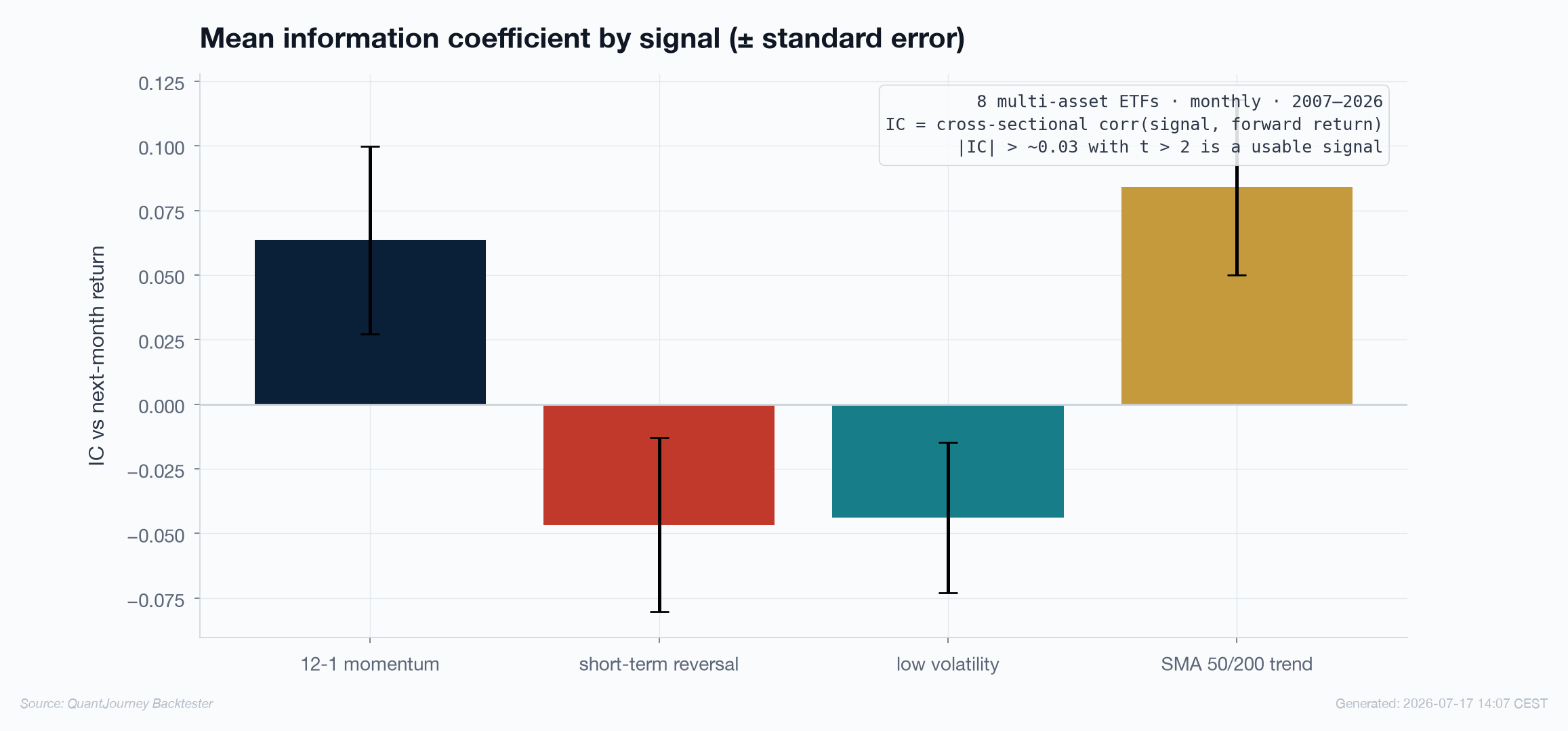
Read the table as a descriptive screen, not a final verdict. Under the unadjusted i.i.d. calculation, SMA trend is the only row below 0.05 (t = 2.48, raw p = 0.014); after Holm correction across the four displayed signals its adjusted p-value is approximately 0.056, before any HAC adjustment. Twelve-month momentum lands at t = 1.75 (raw p = 0.081) on this universe and sample — suggestive, not established. That is not a refutation of momentum; eight assets over eighteen years is a thin test. The IC hit rate remains descriptive: 57–58% for the two trend-family estimates and below 50% for reversal and low volatility.
Grinold's fundamental law of active management explains how a 0.08 IC becomes real money. The information ratio of a strategy scales as IC times the square root of breadth — the number of independent bets:
A 0.08 IC applied repeatedly can be a different proposition from the same IC applied once, but breadth means the number of independent bets — not assets multiplied mechanically by dates. Cross-asset correlation and overlapping information reduce effective breadth. This is also why a signal's IC must be stable across names and time, not concentrated in one lucky asset or regime. Which is the next question.
Stability: is the edge there all the time, or was it one regime?
A mean IC hides its own history. A signal that averaged 0.08 by being +0.30 in 2009 and zero since is not the same asset as one that held 0.08 throughout — and only the second is tradeable going forward.
The rolling IC exposes this directly: a trailing window of the IC series shows when the signal worked and when it went quiet. Alongside it, two summary numbers matter — IC volatility (the denominator of ICIR; high vol means an unreliable edge even at the same mean) and IC stability across regimes (does the sign survive in crisis vs calm, in rates-up vs rates-down?).
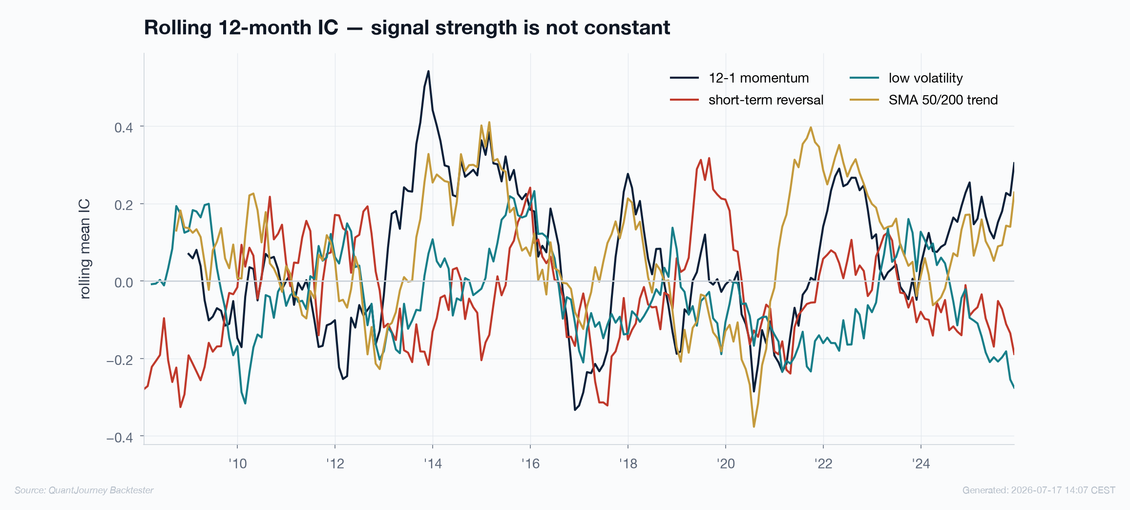
This chart is the honest antidote to a single flattering number. The trend signal has the strongest positive average here, but the current raw test does not establish family-wise significance; its observed contribution is also episodic. A signal whose rolling IC never leaves its home half-plane would support more confidence than any of these four, which is why the sizing layer and the luck-vs-skill gates are the rest of the argument.
Lead-IC decay: how fast does the edge age?
Predictive power is not a constant — it fades as the target moves further into the future. How fast it fades sets your rebalance clock and your capacity.
Measure the IC of today's signal against the single-period return observed h months ahead, for a ladder of h. This is a lead-IC profile, not the cumulative return from today through h. If an exponential decay model is fitted and supported by the data, its half-life is:
# IC decay: correlate the signal with the single-period return h
# months ahead. As h grows, a decaying edge fades toward zero.
horizons = [1, 2, 3, 6, 9, 12]
decay = {h: cross_sectional_ic(signal, me.pct_change().shift(-h)).mean()
         for h in horizons}

# 12-1 momentum:  0.063 -> 0.043 -> 0.025 -> 0.042 -> 0.014 -> 0.002
#   first falls below half at h=3; the profile is non-monotonic,
#   so this is not a fitted exponential half-life
# SMA trend:      0.084 -> 0.072 -> 0.074 -> 0.050 -> 0.036 -> 0.019
#   first falls below half near h=9; no lambda is fitted here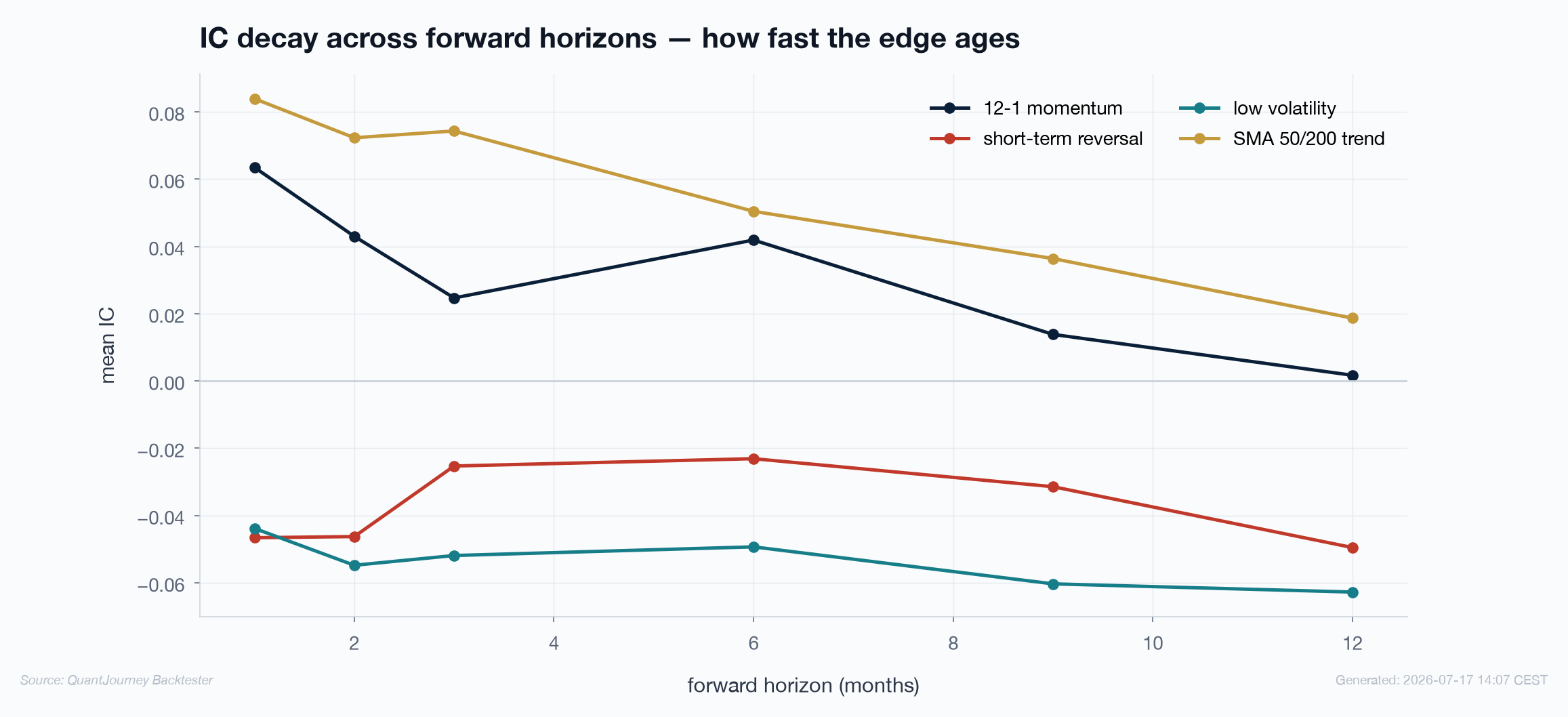
The lead-IC profile is a useful input to the rebalance decision, not a clock by itself. Momentum's early decline suggests testing a faster cadence than SMA trend, but the non-monotonic points do not identify a precise optimal frequency. Rebalancing must be selected jointly with turnover, costs and stability: trade much faster than the useful lead profile and you may pay for little additional information; trade too slowly and the observed relation may fade before execution. A precise half-life claim would require fitting the decay model, reporting uncertainty around lambda and checking that the exponential specification is credible.
Which signal is actually doing the work?
When several signals feed one model, IC grades each in isolation. Permutation importance grades them in combination — how much predictive power the model loses when one signal is scrambled.
The method is model-agnostic and simple: fit a predictor of the forward return, record its R² on a specified evaluation set, then shuffle one feature column in that set and re-score. The drop measures how much that fitted model relied on the feature on that evaluation set. The example below reuses the estimation sample, so it is descriptive in-sample attribution rather than evidence of generalization:
# Model-agnostic permutation importance: fit ANY predictor of the
# forward return, then shuffle one feature column and measure the drop
# in estimation-sample R². This describes reliance inside the fitted sample;
# it does not measure out-of-sample generalization.
from sklearn.linear_model import LinearRegression

X = panel[["mom_12_1", "st_rev", "lo_vol", "trend"]].to_numpy()
y = panel["fwd_return"].to_numpy()
model = LinearRegression().fit(X, y)
base = model.score(X, y)

rng = np.random.default_rng(42)
importance = {}
for j, name in enumerate(features):
    drops = []
    for _ in range(30):
        Xp = X.copy(); Xp[:, j] = rng.permutation(Xp[:, j])
        drops.append(base - model.score(Xp, y))
    importance[name] = np.mean(drops)

# pooled in-sample monthly R² = 0.005
# ranking:  trend 0.0135  >  momentum 0.0077  >  reversal 0.0033  >  lo-vol 0.0013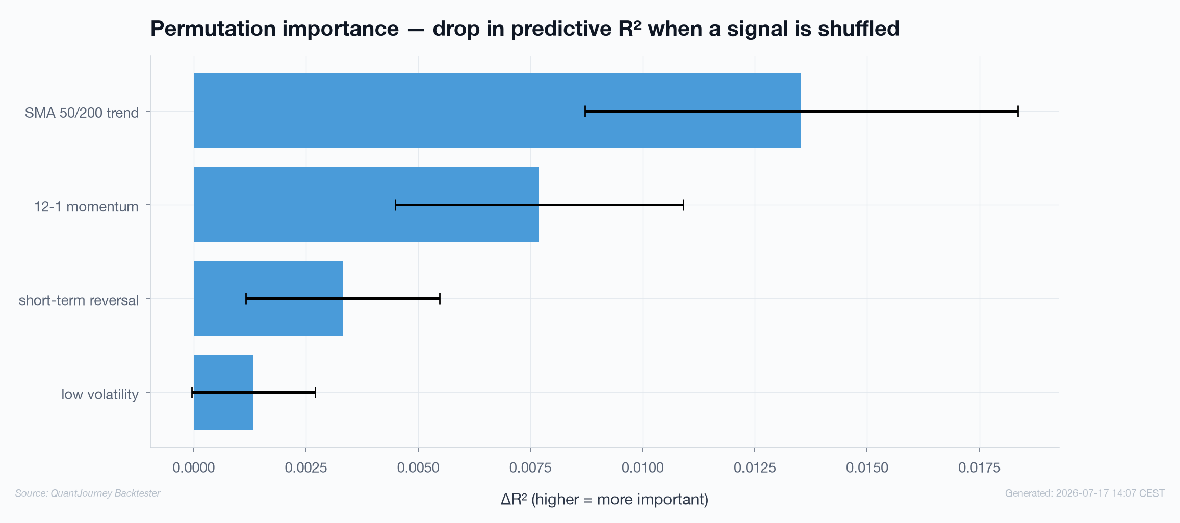
Three caveats keep this from being oversold. First, the pooled in-sample R² is 0.005: the fitted model accounts for half a percent of estimation-sample variation, not out-of-sample return variance. Second, permutation importance is model-relative — a gradient-boosted tree can rank features differently because it can use interactions the linear model cannot. Third, shuffling pooled panel rows ignores date and time structure. A generalization claim requires blocked or walk-forward folds, permutation only in each held-out fold, and a scheme appropriate to the panel hypothesis — for example within-date shuffling for cross-sectional content.
When you bring an actual machine-learning model, richer attribution becomes available: SHAP values allocate a single prediction's output across its features with game-theoretic consistency, and SAGE extends that to global feature importance under interactions. They are richer than a single global permutation score — and strictly dependent on the fitted model and evaluation design. This example provides an in-sample model-inspection floor. Generalization still has to be established on held-out time folds before any attribution method answers the production question: which inputs does the forecast reliably use on unseen data?
Grading a signal before it becomes a strategy
Six numbers decide whether a signal is worth building a strategy around. Compute them first; they are cheap, and they retire most ideas before the expensive stages.
Mean IC on the right scale
Treat 0.05–0.10 monthly as a context-dependent research heuristic, not a universal pass mark. Rank IC alongside Pearson IC for robustness to outliers and monotone transformations.
Dependence-robust, family-aware inference
Report the raw i.i.d. statistic only as a diagnostic. Use HAC or a time-block bootstrap and correct the pre-declared signal family for multiple testing; none of the four displayed rows clears Holm-adjusted 5% on the current raw p-values.
ICIR with its assumptions visible
The Sharpe-like ratio of the IC series. Its √12 annualization is descriptive when monthly IC is serially dependent, so inspect the dependence rather than treating ICIR as assumption-free.
Rolling IC stays on its side
Read the whole history, not the average. An edge concentrated in one regime is a regime bet wearing a signal costume.
Lead-IC profile informs the rebalance clock
Use the empirical profile with turnover and costs. Call a number “half-life” only after fitting and validating a decay model; the current chart reports first half-value crossings instead.
Effective breadth × IC, then validate
A small IC needs independent breadth to matter; correlated assets and overlapping dates do not count as separate bets. The skill-vs-luck gates and walk-forward decide whether it survives as a strategy.
References
- Grinold, R. C. & Kahn, R. N. (2000). Active Portfolio Management, 2nd ed. — the information coefficient, ICIR and the fundamental law of active management.
- Grinold, R. C. (1989). The Fundamental Law of Active Management. Journal of Portfolio Management 15(3) — IR ≈ IC · √breadth.
- Jegadeesh, N. & Titman, S. (1993). Returns to Buying Winners and Selling Losers. Journal of Finance 48(1) — cross-sectional momentum.
- Newey, W. K. & West, K. D. (1987). A Simple, Positive Semi-definite, Heteroskedasticity and Autocorrelation Consistent Covariance Matrix. Econometrica 55(3) — dependence-robust standard errors.
- Holm, S. (1979). A Simple Sequentially Rejective Multiple Test Procedure. Scandinavian Journal of Statistics 6(2) — family-wise multiple-testing control.
- Lundberg, S. & Lee, S.-I. (2017). A Unified Approach to Interpreting Model Predictions. NeurIPS — SHAP values.
- Covert, I., Lundberg, S. & Lee, S.-I. (2020). Understanding Global Feature Contributions With Additive Importance Measures. NeurIPS — SAGE.
- Breiman, L. (2001). Random Forests. Machine Learning 45(1) — permutation importance.