Same signal, different portfolio
Once the signal says what to hold, everything that determines how the portfolio actually behaves — its volatility, its drawdowns, which crisis hurts it — is decided by how much of each position you hold. This guide works through the four canonical sizing schemes in risk units: the math of each, the failure mode of each, and the engine's pluggable risk-model layer that lets one line of config switch between them. Then it runs one trend signal through all five configurations on nineteen years of real data and lets 2008, 2020 and 2022 grade the schemes — each of which flatters a different one.
Sizing is a decision you are already making
Equal weight is not the absence of a sizing scheme. It is a specific one — with a specific, measurable risk profile that most people never look at.
The experiment for this whole guide: take the SMA(50/200) trend basket from the workflow guide — eight multi-asset ETFs, long the trending ones, equal weight, monthly rebalance, 5 bps per side, 2007–2026 — and change only the sizing layer. Same signal, same dates, same costs, and the same daily rescore calendar on every model, five portfolios:
SIZINGS = [
    ("Equal weight",        None),
    ("Inverse vol",         InverseVolModel(lookback=63, blend_alpha=False)),
    ("Vol target 10%",      VolTargetModel(target_vol=0.10, lookback=63,
                                           max_leverage=1.5, rebalance_freq="D")),
    ("Risk parity (ERC)",   RiskParityModel(lookback=63, rebalance_freq="D")),
    ("Institutional chain", RiskModelChain([
                                RiskParityModel(lookback=63, rebalance_freq="D"),
                                VolTargetModel(target_vol=0.10, lookback=63,
                                               max_leverage=1.5, rebalance_freq="D"),
                                PositionLimitModel(max_weight=0.30,
                                                   max_total_leverage=1.5),
                            ])),
]

# Pin every model to a DAILY rescore so all five read an equally fresh
# estimate (inverse vol already rescores every bar; ERC and vol target
# default to monthly). RebalancePolicy(BME) stays the single execution
# clock, so only the sizing math differs across the five rows.
for label, model in SIZINGS:
    s = TrendBasket(..., risk_model=model)    # NOTHING else changes
    await s.run_strategy()
The ERC and Institutional Chain results shown below were generated using the hosted exact-ERC solver. Results from the open-source iterative implementation may differ slightly.
| Sizing | CAGR | Vol | Sharpe | Max DD | Worst month | Turnover | Avg gross |
|---|---|---|---|---|---|---|---|
| Equal weight | 5.11% | 10.91% | 0.512 | −22.2% | −8.3% | 3.4× | 0.89 |
| Inverse vol | 4.80% | 9.57% | 0.538 | −22.1% | −8.0% | 3.6× | 0.89 |
| Vol target 10% | 5.37% | 10.54% | 0.550 | −28.9% | −12.4% | 3.8× | 0.94 |
| Risk parity (ERC) | 4.82% | 9.11% | 0.563 | −21.7% | −8.0% | 3.9× | 0.89 |
| Institutional chain | 5.73% | 10.68% | 0.576 | −25.0% | −8.9% | 3.7× | 1.01 |
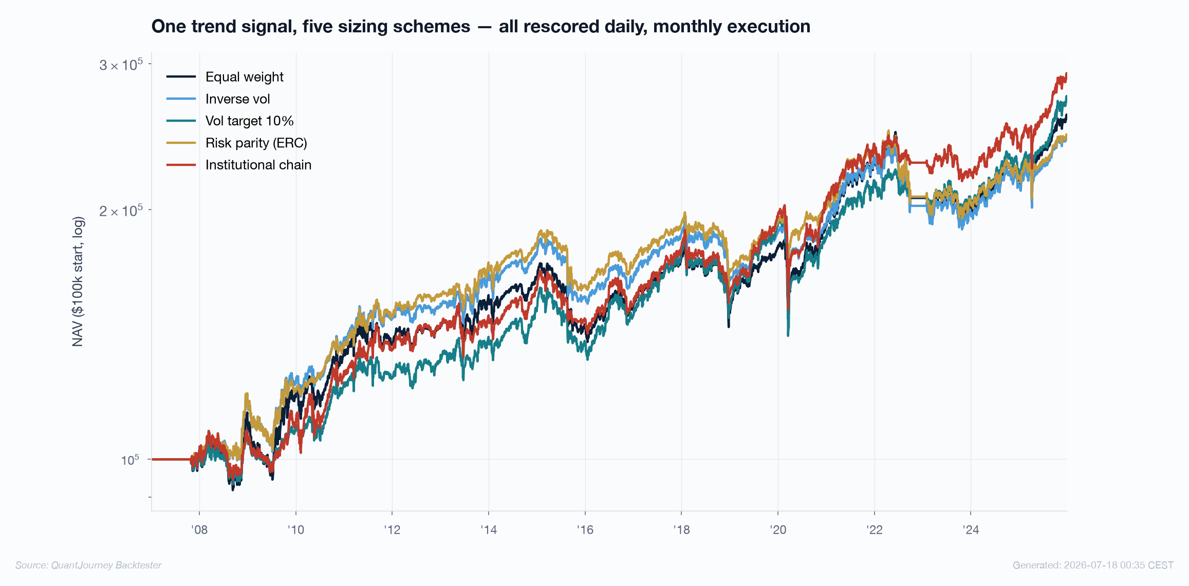
risk_model= argument — every
scheme rescored daily and executed monthly, so nothing but the sizing math moves. The spread — 4.8% to 5.7%
CAGR, −21.7% to −28.9% max drawdown — is pure sizing.
Read the spread before reading any single row: the gap between the best and worst configuration is 0.9 points of CAGR and 7 points of drawdown — from the same signal. That is a larger performance difference than most signal "improvements" deliver, and it is available without touching the alpha at all. The rest of this guide explains each row: what the scheme optimizes, what it silently assumes, and which of the three crises in the sample called its bluff.
Where sizing lives in the engine
Sizing is a pipeline stage, not a strategy rewrite: signals → weights → risk model → rebalance policy → execution.
The strategy's _compute_weights() returns raw conviction — what the signal wants to own. The risk
model receives those targets together with the asset return history and reshapes them; the
rebalance policy then decides on which dates the reshaped targets become
trades. Keeping the layers separate is what made the five-run experiment above a five-line change — and what
makes sizing schemes comparable at all, because everything else is held fixed by construction:
from backtester.risk.base import RiskModel

class RiskModel(abc.ABC):
    @abc.abstractmethod
    def adjust(
        self,
        weights: pd.DataFrame,     # raw targets from _compute_weights()
        returns: pd.DataFrame,     # daily asset returns, same shape
        *,
        metadata: dict | None = None,
    ) -> pd.DataFrame:
        """Adjust weights given historical returns."""

# The contract every model honors:
#  1. Estimates use STRICTLY PRIOR windows - returns[i-lookback : i]
#     never includes bar i. Sizing cannot look ahead.
#  2. A model may RESIZE positions, never CREATE them - an instrument
#     the signal left at zero stays at zero.
#  3. Total exposure is preserved unless changing it is the model's
# entire point (vol targeting).Every estimate a risk model consumes — per-asset vol, portfolio vol, the covariance matrix — is computed on a window that ends strictly before the bar being sized. The same decide-at-t-earn-at-t+1 discipline the workflow guide demands of signals applies to sizing, because a sizing layer that peeks is just look-ahead wearing a risk costume.
Reading a portfolio in risk units
Capital weights answer "where is the money?" Risk contributions answer "where is the pain?" The two pictures disagree far more than intuition expects.
Portfolio volatility decomposes exactly — not approximately — into per-asset contributions. This is Euler's theorem applied to σp: each asset's contribution is its weight times its marginal effect on portfolio risk, and the contributions sum to the total:
Dividing by σp once more gives shares that sum to one. A share can be negative — an asset negatively correlated with the rest of the book removes risk even while consuming capital:
Now apply this lens to the plain equal-weight eight-ETF basket, using the realized 2007–2026 covariance. Capital says "12.5% each, nicely diversified". Risk says something else entirely:
| Asset | Ann. vol | RC share — equal weight | RC share — inverse vol | ERC weight | RC share — ERC |
|---|---|---|---|---|---|
| SPY (US equity) | 19.8% | 16.6% | 16.7% | 8.3% | 12.5% |
| EFA (intl equity) | 21.7% | 18.9% | 17.7% | 7.0% | 12.5% |
| EEM (EM equity) | 28.0% | 24.2% | 17.4% | 5.6% | 12.5% |
| TLT (20y+ bonds) | 15.2% | −0.8% | 4.0% | 17.3% | 12.5% |
| IEF (7–10y bonds) | 7.0% | −0.3% | 4.6% | 35.3% | 12.5% |
| GLD (gold) | 17.5% | 6.7% | 11.0% | 10.8% | 12.5% |
| DBC (commodities) | 19.2% | 11.2% | 12.9% | 10.2% | 12.5% |
| VNQ (REITs) | 29.8% | 23.5% | 15.8% | 5.5% | 12.5% |
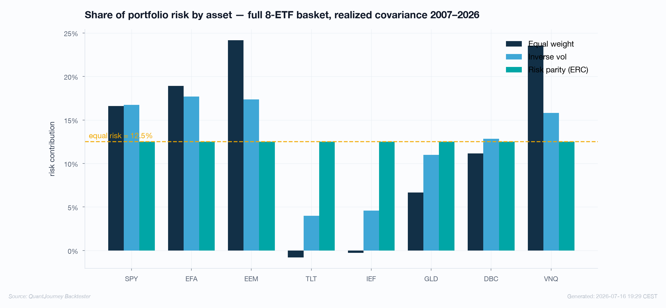
Three readings. The equal-weight basket is an equity portfolio wearing a diversified costume: SPY, EFA, EEM and VNQ carry 83% of the risk. The bonds' shares are negative — over this sample TLT and IEF hedged the book more than they risked it, so in risk terms the "12.5% capital each" story was fiction on both ends. And the ERC column shows what actually equalizing risk requires: over half the capital (52.6%) in the two bond ETFs, with the three most volatile assets cut to 5–8% each. No intuition produces those numbers; a covariance matrix does.
Inverse volatility — the first risk budget
One estimate per asset, no matrix: capital inversely proportional to each asset's own volatility.
from backtester.risk import InverseVolModel

strategy = TrendBasket(
    ...,
    risk_model=InverseVolModel(
        lookback=63,          # trailing window for per-asset vol
        min_vol=0.01,         # floor - prevents 1/sigma blowups
        blend_alpha=False,    # False: pure 1/vol among active assets
                              # True:  raw_weight x 1/vol, renormalized
                              #        (conviction x risk adjustment)
    ),
)
Inverse vol equalizes standalone risk: if every pairwise correlation were identical, it would be exact ERC. Its virtue is robustness — n vol estimates instead of n(n+1)/2 covariance entries — and the table above shows it doing real work: EEM's risk share drops from 24.2% to 17.4%, the bonds' rise from negative to positive. Its blind spot is the correlation structure: it cannot see that the equity block co-moves, so it still grants the block two thirds of the total risk.
The measured run makes the blind spot concrete. Inverse vol delivered the intended vol reduction (9.4% vs 10.9% for equal weight) — and a worse drawdown: −26.7%, peaking March 2022 and bottoming October 2023. The scheme's bond tilt was calibrated on the pre-2022 regime, where bond vol was low and bond-equity correlation was negative. In 2022 rates repriced, the correlation flipped positive, and the "low-risk" sleeve became the epicenter — while the vol estimates, trailing 63 days behind, kept feeding it capital. A sizing scheme is a bet on the stability of its own inputs; inverse vol bets on two of them at once.
Volatility targeting — sizing the whole book
The previous schemes decide the shape of the portfolio. Vol targeting decides its level: one scalar, applied to everything, so realized volatility tracks a chosen target.
from backtester.risk import VolTargetModel

strategy = TrendBasket(
    ...,
    risk_model=VolTargetModel(
        target_vol=0.10,       # annualized portfolio target
        lookback=63,           # trailing window for realized vol
        max_leverage=1.5,      # hard cap on the scale factor
        rebalance_freq="D",    # how often to RE-ESTIMATE the scale
    ),
)

# Two clocks, not one: this rebalance_freq re-estimates the scale, but the
# book only MOVES when RebalancePolicy fires a trade. The slower clock wins
# — which is the entire story of the COVID chart below.
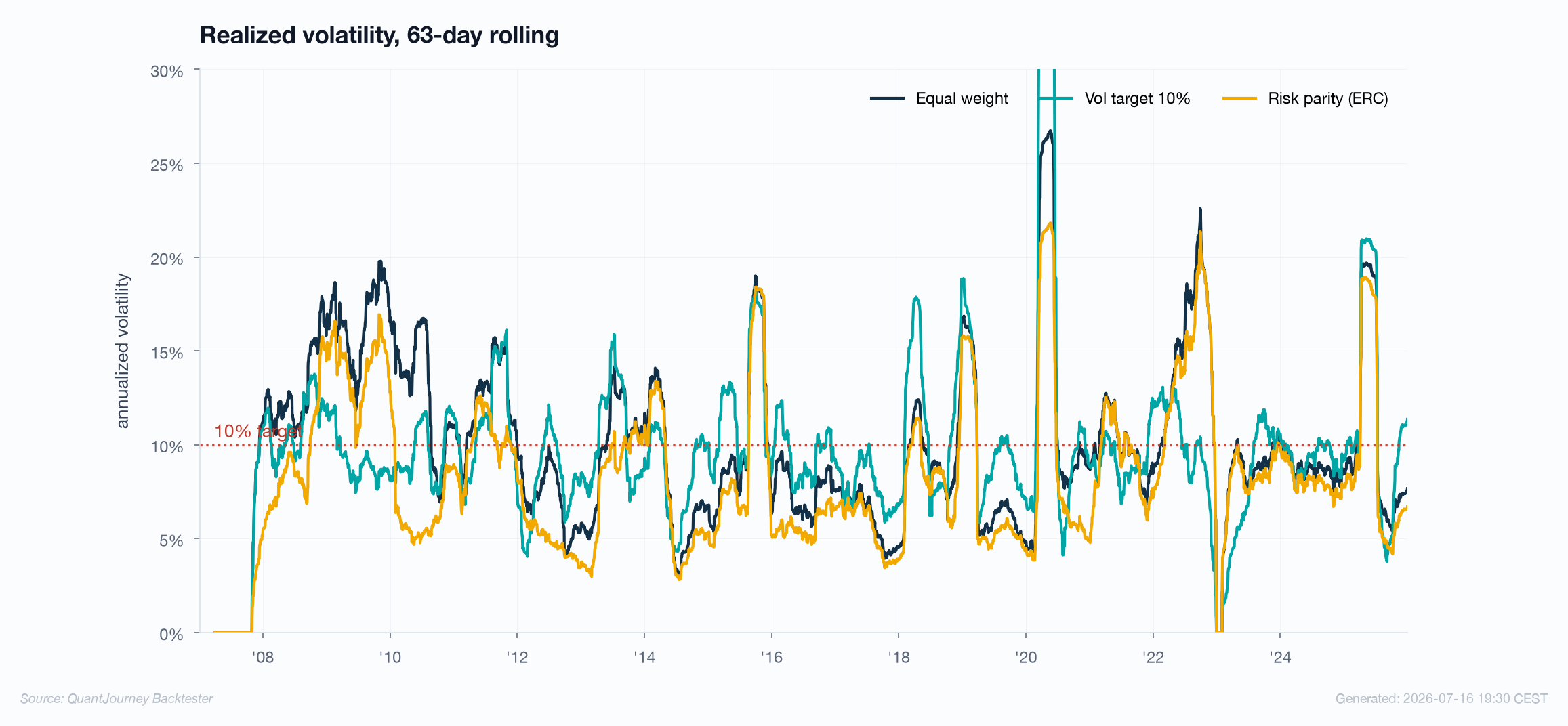
The promise is a portfolio that leans in when markets are calm and de-risks when they are turbulent — and across regimes, it delivers: the rolling-vol chart below shows the teal line hugging the 10% target through the long calm stretches where equal weight wanders between 6% and 18%. The trap is hiding in the word "trailing". The scale st is an estimate of the recent past, held until the next rescore. When volatility jumps, the scheme is — by construction — positioned for the world that just ended.
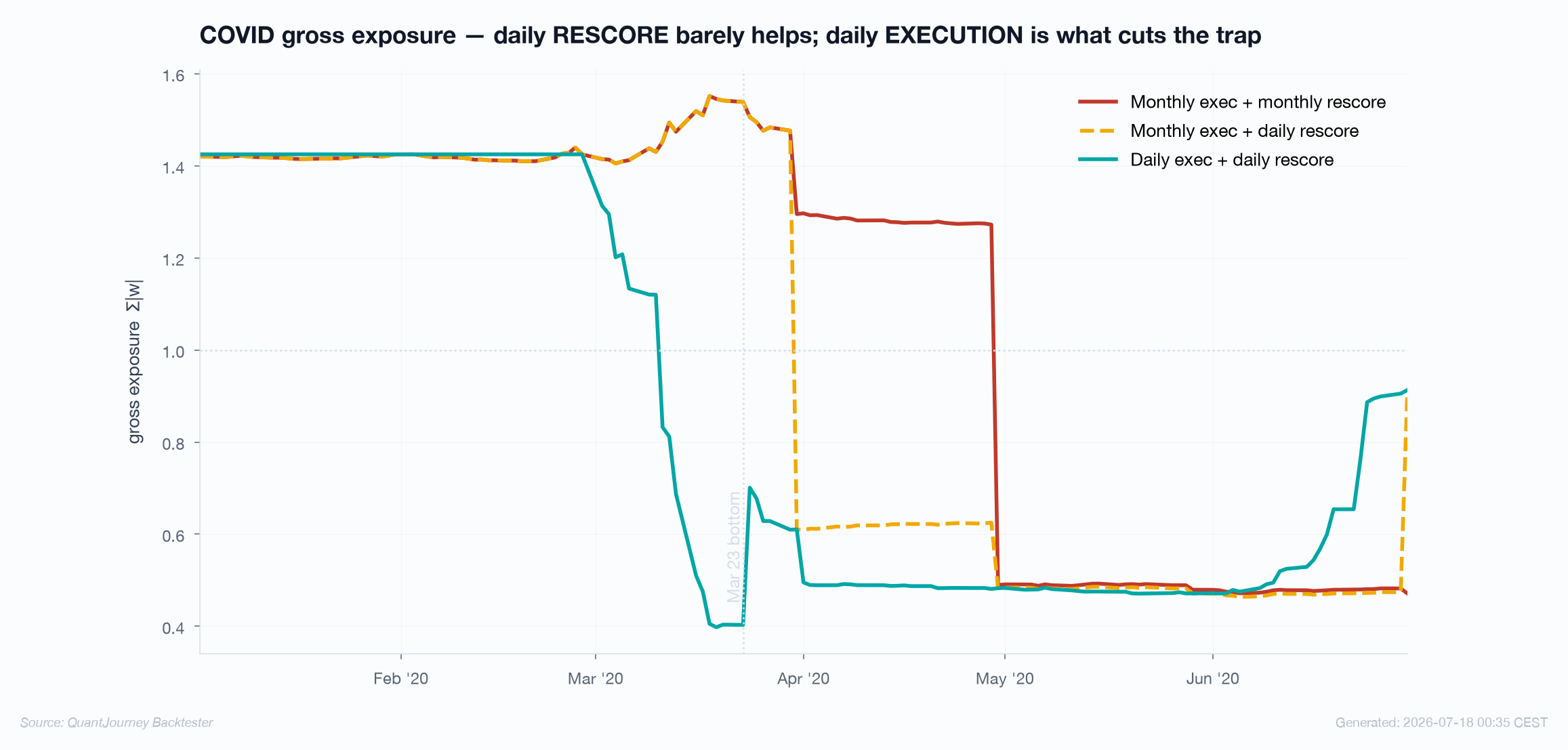
It is tempting to blame the monthly rescore — the scale was set on stale data. The engine says otherwise. Run the identical vol target three ways and the cause separates cleanly into three distinct lags:
| Configuration | Gross, Feb 19 | Gross, Mar 23 (bottom) | Max DD | Worst month |
|---|---|---|---|---|
| Monthly execution + monthly rescore | 1.41× | 1.54× | −28.9% | −12.4% |
| Monthly execution + daily rescore | 1.41× | 1.54× | −28.9% | −12.4% |
| Daily execution + daily rescore | 1.42× | 0.40× | −19.4% | −8.5% |
Three lags, and only one of them matters here. Estimation lag is irreducible: even the
daily/daily book enters the crash at 1.42×, because a 63-day window cannot price a volatility spike that has not
happened yet — no configuration escapes that first column. Model-refresh lag — how often the
risk model recomputes its target — is the dial people reach for first, and the top two rows show it does
nothing here: a daily rescore under monthly execution is bit-for-bit identical to a monthly rescore
straight through the crash. Execution lag is the entire effect: the position only moves when
RebalancePolicy fires, so under monthly rebalancing the levered February book is frozen through the
March collapse. Switch execution to daily and the same target deleverages during the fall — max
drawdown −28.9% → −19.4%, worst month −12.4% → −8.5% — at the cost of turnover and whipsaw.
So the lesson is sharper than "estimation takes time". Vol targeting stabilizes regime volatility and
cannot anticipate the transition into a crisis — that part is estimation lag, and it is real and
irreducible. But the deepest drawdown in this experiment, in its shortest window (peak February 21,
trough March 18, 2020), was manufactured by the rebalance calendar, not the estimator. A faster
rebalance_freq on the risk model would not have touched it; a faster execution policy would have.
Name which lag you are looking at before you reach for a dial — two of the three here move the wrong one.
Risk parity — equal risk, actually equal
ERC is inverse vol upgraded with the full covariance matrix: every asset contributes the same share of portfolio risk, correlations included.
Unlike the closed-form schemes, ERC weights have no explicit formula — they are the solution of a fixed-point problem. The hosted QJ Backtester solves Spinu's convex formulation using a damped Newton method, producing equal-risk-contribution weights to numerical tolerance. The open-source package includes a lightweight iterative approximation, while exact ERC is available in the hosted engine:
from backtester.risk import RiskParityModel

strategy = TrendBasket(
    ...,
    risk_model=RiskParityModel(
        lookback=63,     # trailing covariance window
        max_iter=50,     # solver iteration cap
        tol=1e-8,
    ),
)

# Results in this guide use the hosted exact-ERC solver. The open-source
# implementation uses a lightweight iterative approximation, so its
# numerical results may differ slightly.
In the measured run, ERC is the honest defensive scheme in the lineup: the lowest volatility (9.25%), the shallowest drawdown (−21.6%), the mildest worst month (−8.0%), and — unlike inverse vol — it earned its lower risk without the 2022 faceplant, because the covariance window saw the correlation flip and rebalanced the risk budget away from the failing hedge. The price: a Sharpe only 0.04 above equal weight, moderate extra turnover (3.9× vs 3.4×) from tracking a moving covariance, and — the structural one — a lower expected return, because equalizing risk means allocating away from the highest-premium assets. ERC buys smoothness, not alpha. Whether that trade is good depends on what the smoothness is for — which is the chain's question.
Position limits — the compliance floor
Whatever the statistical schemes propose, hard constraints dispose. Caps, floors, leverage and sector limits run last, so the final book respects them no matter what produced it.
from backtester.risk import PositionLimitModel

limits = PositionLimitModel(
    max_weight=0.30,             # per-instrument cap
    min_weight=0.02,             # floor for ACTIVE positions (0 = off)
    max_total_leverage=1.5,      # cap on sum(|w|)
    sector_limits={"equity": 0.60, "rates": 0.50},
)

# Sector caps need a sector map in metadata:
#   metadata={"sectors": {"SPY": "equity", "TLT": "rates", ...}}
# Excess above a cap is redistributed proportionally among uncapped
# active instruments, iteratively, so total exposure survives intact.
The redistribution detail matters: naive capping (clip and renormalize everything) leaks exposure back into the
capped names. The engine caps iteratively — excess is redistributed only among instruments with headroom, and
the loop repeats until no cap is breached, so a 30% cap means 30%, exactly, while total exposure survives. The
same model quietly powers the max_position_size= constructor argument: in weights mode the engine
routes it into a PositionLimitModel, so the cap is enforced accounting, not a report label.
Composing the stack
The schemes are orthogonal decisions — shape, level, constraints — and the engine composes them in one chain, output of each feeding the next.
from backtester.risk import (
    PositionLimitModel, RiskModelChain, RiskParityModel, VolTargetModel,
)

strategy = TrendBasket(
    ...,
    risk_model=RiskModelChain([
        RiskParityModel(lookback=63),                  # 1. shape: equal risk
        VolTargetModel(target_vol=0.10, lookback=63,   # 2. level: 10% vol,
                       max_leverage=1.5),              #    lever if needed
        PositionLimitModel(max_weight=0.30,            # 3. compliance: caps
                           max_total_leverage=1.5),    #    bind LAST
    ]),
)

# Order is semantics, not style:
#   ERC -> VolTarget:  target the vol of the DIVERSIFIED book
#   VolTarget -> Limits: caps clip whatever leverage produced
# Reversed, the chain answers a different question.
This is the standard institutional construction — risk parity funds and managed-futures books are variations of exactly this stack — and the measured result shows why: Sharpe 0.576 and 5.73% CAGR, the best of the experiment. The mechanism is visible in the "avg gross" column of the headline table: the ERC book runs at 9.11% vol, well under the 10% target, so the vol-target stage levers it (average gross exposure 1.01, peaks at 1.5×) — spending the risk budget that ERC's diversification freed up. Leverage applied to a genuinely diversified book is the one free-ish lunch in this guide.
And the honest cost, in the same table: the chain's drawdown is −25.0%, three points deeper than pure ERC, and its worst month −8.9% — the vol-target stage's crisis exposure, inherited. Each overlay solves the problem the previous one left and introduces its own; the composition is better on the average day and worse on the worst day than its most defensive component. That is not a flaw to engineer away — it is the actual shape of the trade-off, and the reason the stack must be measured as a whole rather than reasoned about one layer at a time.
Estimation risk is the hidden parameter
Every scheme above replaced the question "how much do I hold?" with "how well can I estimate risk?" That trade has terms and conditions.
All four schemes consume estimates — a vol, a covariance — computed on a trailing window, and the window length
is a real parameter with a real trade-off: short windows (21–63 days) adapt fast and whipsaw on noise; long
windows (252+) are stable and permanently late. The measured runs used 63 days throughout — but the two failures
we documented are not the same animal, and conflating them points you at the wrong fix. Inverse vol
feeding the 2022 bond crash is estimation lag proper: the trailing window had simply not seen the regime. Vol
targeting levered into COVID is mostly execution lag — a rebalance-calendar artifact, as the three-way
table above shows, that a faster estimator does nothing for. Estimation lag is irreducible and you manage it;
execution lag is a scheduling choice and you fix it. Three disciplines keep the estimation honest rather than hopeful.
Floors and fallbacks: the engine floors vol estimates (min_vol) so a quiet quarter
cannot produce a 50× position, and degenerate covariances fall back to inverse-vol weights rather than crashing
or fabricating. Strictly prior windows: enforced by the layer's contract, not by author
discipline. And the same statistical bar as the signal: a sizing overlay changes the return
series, so it changes the evidence — the validation gates run on
the sized strategy, and an overlay added after validation invalidates the certificate. Sizing is part of
the process being tested, never a garnish on top of it.
Lookbacks, targets and caps are estimation hygiene, not free parameters. If you optimize
target_vol to maximize the backtest Sharpe, you have added dimensions to the search space, and the
selection-bias corrections must know about every value you
tried. The defensible pattern: fix the risk parameters from mandate and estimation-quality arguments
(a 10% target because the mandate says so; 63 days because shorter is noise), then validate the whole
configuration once.
The sizing checklist
Six questions to answer before the sizing layer is done.
Look at the book in risk units
Compute RC shares. If one asset class carries 80% of the risk, you own a concentrated portfolio wearing a diversified costume — decide deliberately whether that is intended.
Pick shape and level separately
Shape (EW / inverse vol / ERC) and level (vol target, leverage cap) are different decisions with different failure modes. Choose each on its own merits; compose them in the chain.
Stress the scheme in the regime that breaks it
Inverse vol: correlation flips (2022). Vol targeting: vol spikes from calm (2020). ERC: premium concentration. Every scheme has one; make sure your sample contains it.
Mind the estimation lag
Whatever the lookback, the scheme is positioned for the recent past. Ask what happens in the first month of a regime it has not seen — that is where its worst month lives.
Cap what must never happen
Statistical schemes propose;
PositionLimitModeldisposes. Per-name caps, leverage caps and sector limits run last in the chain, always.Validate the sized strategy
The overlay changes the return series, so the statistical gates run on the final configuration — sizing included, costs included.
We do independent validation engagements — permutation tests, walk-forward, Sharpe selection diagnostics, canonical CSCV context and rolling rank stability on your code or track record, delivered as a signed, reproducible report.
References
- Maillard, S., Roncalli, T. & Teïletche, J. (2010). The Properties of Equally Weighted Risk Contribution Portfolios. Journal of Portfolio Management 36(4) — existence, uniqueness and the vol ordering EW ≥ ERC ≥ min-var.
- Roncalli, T. (2013). Introduction to Risk Parity and Budgeting. Chapman & Hall — the standard reference for risk budgeting mathematics.
- Spinu, F. (2013). An Algorithm for Computing Risk Parity Weights. SSRN 2297383 — the convex formulation the hosted solver minimizes.
- Griveau-Billion, T., Richard, J.-C. & Roncalli, T. (2013). A Fast Algorithm for Computing High-Dimensional Risk Parity Portfolios. SSRN 2325255 — coordinate-descent and Newton approaches to the same problem.
- Moreira, A. & Muir, T. (2017). Volatility-Managed Portfolios. Journal of Finance 72(4) — the case for vol scaling across factor portfolios.
- Harvey, C., Hoyle, E., Korgaonkar, R., Rattray, S., Sargaison, M. & van Hemert, O. (2018). The Impact of Volatility Targeting. Journal of Portfolio Management 45(1) — where vol targeting helps (risk assets) and where it does not.
- DeMiguel, V., Garlappi, L. & Uppal, R. (2009). Optimal Versus Naive Diversification: How Inefficient is the 1/N Portfolio Strategy? Review of Financial Studies 22(5) — why equal weight is a hard benchmark to beat.