Search efficiently. Validate separately.
An optimizer answers one question — which of the configurations I tried scored best on this history — and creates another: is that maximum anything more than the luck of forty draws? This guide covers both halves on real runs: the engine's Optuna integration (typed spaces, TPE, pruning, constraints), a measured TPE-versus-random head-to-head, the Deflated Sharpe Ratio that judges the winner against its own trial count, and the nested walk-forward pattern that makes an optimized strategy's OOS claim honest.
Optimization is two problems, not one
Finding a good configuration is a search problem. Believing the number it reports is a statistics problem. Tools that solve the first while ignoring the second manufacture false discoveries at scale.
Every trial you evaluate raises the bar the winner must clear, whether or not the trial "worked". The expected maximum of N independent zero-skill scores grows like √(2 ln N) — forty trials of pure noise hand their best draw nearly three standard deviations of apparent edge for free:
So this guide treats the optimizer and the corrections as one workflow: search with Optuna (efficiently, reproducibly, every trial logged), then judge the winner with the Deflated Sharpe Ratio against the full trial population, and validate it out of sample — ideally with the search nested inside the folds, which the engine supports natively. Skipping the second half does not make it unnecessary; it makes it your broker's problem to teach you.
The engine wiring: spaces, samplers, constraints
One factory call declares the whole search: typed parameter space, sampler, pruner, seed and validity constraints.
from backtester.walkforward.optimization import optimizer_factory

optimizer = optimizer_factory(
    "optuna",
    param_space={
        "fast": {"type": "int", "low": 10, "high": 80},
        "slow": {"type": "int", "low": 100, "high": 250},
    },
    n_trials=40,
    sampler="tpe",            # or "random" / "grid" / "cmaes"
    pruner="median",          # stop mid-trial when below the running median
    seed=42,                  # the search itself is reproducible
    constraints=[
        {"type": "less_than", "param": "fast", "than": "slow"},
    ],
)

result = optimizer.optimize_fn(evaluate)
result.best_params        # {'fast': 52, 'slow': 141}
result.best_objective     # 0.6928
result.n_evaluated        # 40
result.all_results        # DataFrame: every trial, params x metrics
The objective is an ordinary function: parameters in, one score out — and it is part of the strategy's specification, not plumbing. Three decisions live inside it: the score itself (net Sharpe here — costs on, because the optimizer will happily buy turnover if trades are free), the handling of degenerate trials (no-trade configurations score 0, not NaN), and the defense of invariants (fast < slow returns a penalty even though a constraint also exists — the evaluation function defends itself):
def evaluate(params) -> float:
    """One trial = one full engine backtest, scored net of costs."""
    fast, slow = int(params["fast"]), int(params["slow"])
    if fast >= slow:                      # defend invariants in the objective
        return -999.0                     # even when a constraint also exists

    strategy = build_trend(fast, slow)    # 8 ETFs, BME, 5 bps per side
    asyncio.run(strategy.run_strategy())

    returns = strategy.portfolio_data.net_asset_value.pct_change().dropna()
    if returns.empty or returns.std() == 0:
        return 0.0                        # no-trade degenerate -> neutral score
    return float(returns.mean() / returns.std() * np.sqrt(252))
Grid, random, TPE — the same question, different budgets
Our two-parameter space contains 10,721 valid integer pairs. Enumerating it is honest and unaffordable; sampling it is the entire craft.
Grid search evaluates a pre-declared lattice — complete over what you declared, blind between
the lattice points, and exponential in dimensions. It remains the right tool for small sensitivity surfaces
(the engine ships example_wf_04 with a 3×3 grid). Random search spends its budget
uniformly — no adaptivity, but immune to lattice aliasing. TPE (Tree-structured Parzen
Estimator) is adaptive: after warm-up trials it splits observed results into a "good" set and a "rest" set,
models each as a density, and proposes the candidate that maximizes their ratio — sampling where good results
cluster while keeping exploration alive:
We ran the comparison instead of asserting it — same space, same seed, same 40-trial budget, real engine backtests per trial:
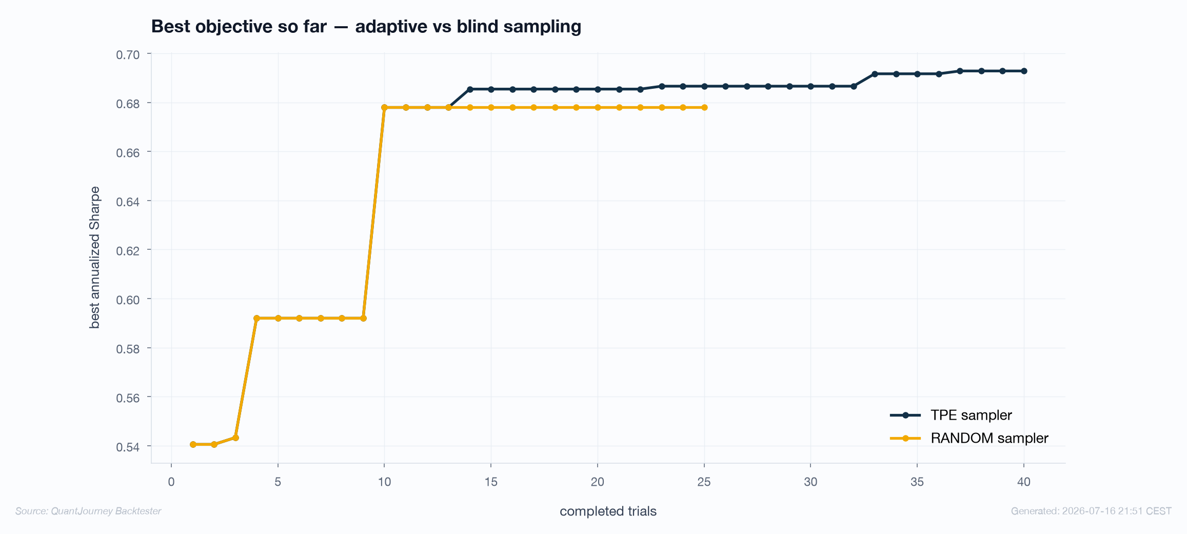
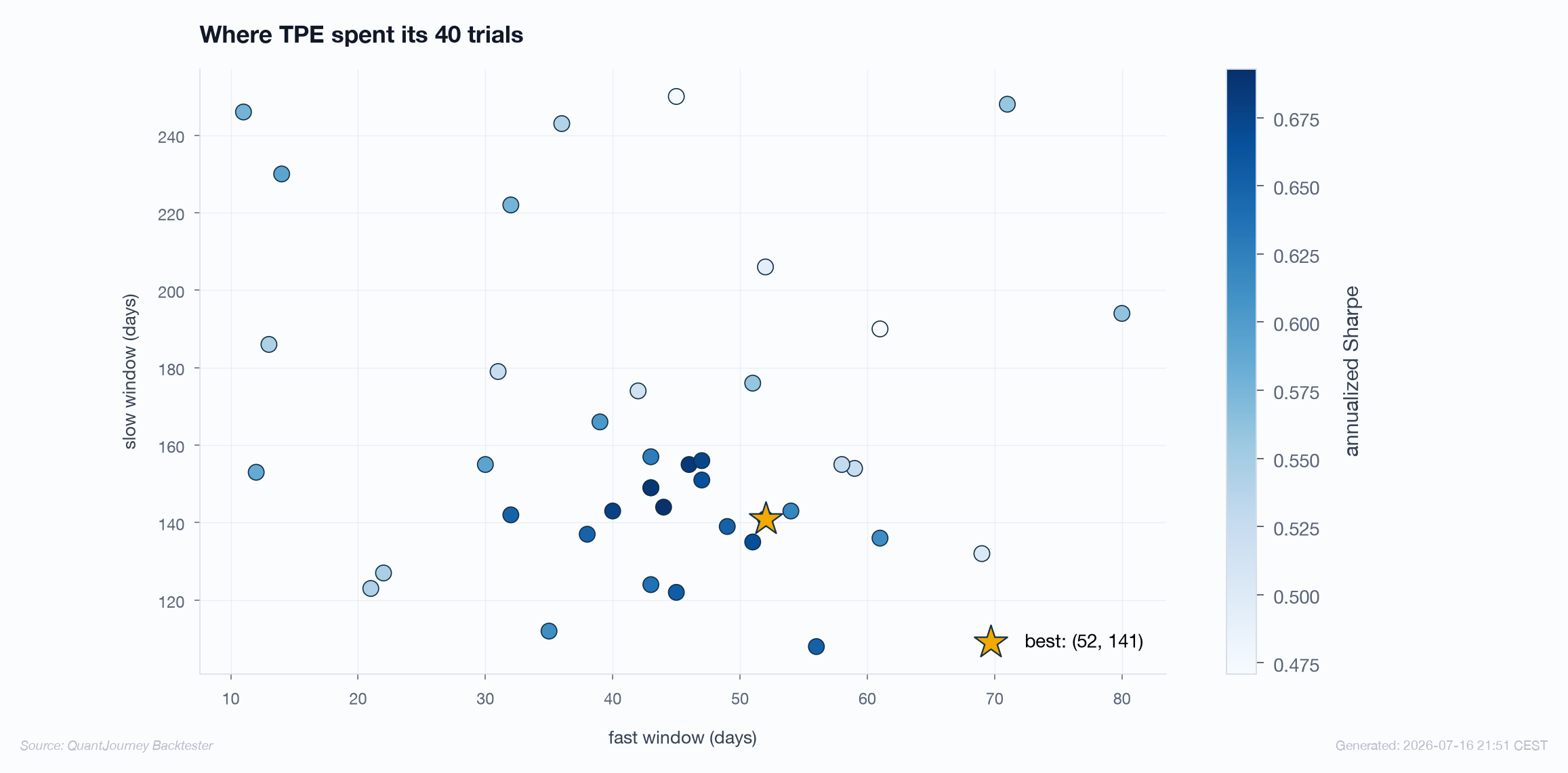
Two honest readings. First, the margin is small — 0.693 vs 0.678 on this smooth two-dimensional surface — because TPE's advantage grows with dimensionality, conditionality and expensive trials; on a 2-D plateau random is a respectable competitor. Second, the constraint accounting matters more than the headline: TPE's proposal model learns the feasible region, while random re-discovers it by dying there, 15 times. On a five-parameter space with real constraints, that difference compounds into most of the budget.
| Grid | Random | TPE | |
|---|---|---|---|
| Coverage | Complete on the declared lattice | Uniform in expectation | Adaptive, concentrates on promise |
| Cost scaling | Product of dimensions | Linear in budget | Linear in budget |
| Constraints | Filtered upfront | Wasted proposals (15/40 here) | Learned; near-zero waste |
| Reproducibility | Deterministic | Seeded | Seeded (seed=42) |
| Removes selection bias? | No | No | No |
Pruning: paying less for bad news
A pruner abandons trials that are clearly losing before they finish — the median rule stops any trial whose running score falls below the median of completed trials at the same stage.
Pruning changes both the search path and the information in the study. A pruned proposal is still part of the
research audit, but without a comparable finite final objective it cannot estimate the cross-trial Sharpe
variance used by DSR. The engine records pruned and failed states so the search history remains honest. The practical rule: enable
pruner="median" whenever single trials are expensive (per-fold refits, intraday data), and keep
the pruned fraction visible in the study audit — a study where 80% of trials were pruned is telling you the
space is mostly dead, which is itself a finding about the hypothesis.
Judging the winner: the maximum is not a draw
The study's best trial earned Sharpe 0.693. The study's median trial earned 0.60. Which number is the strategy?
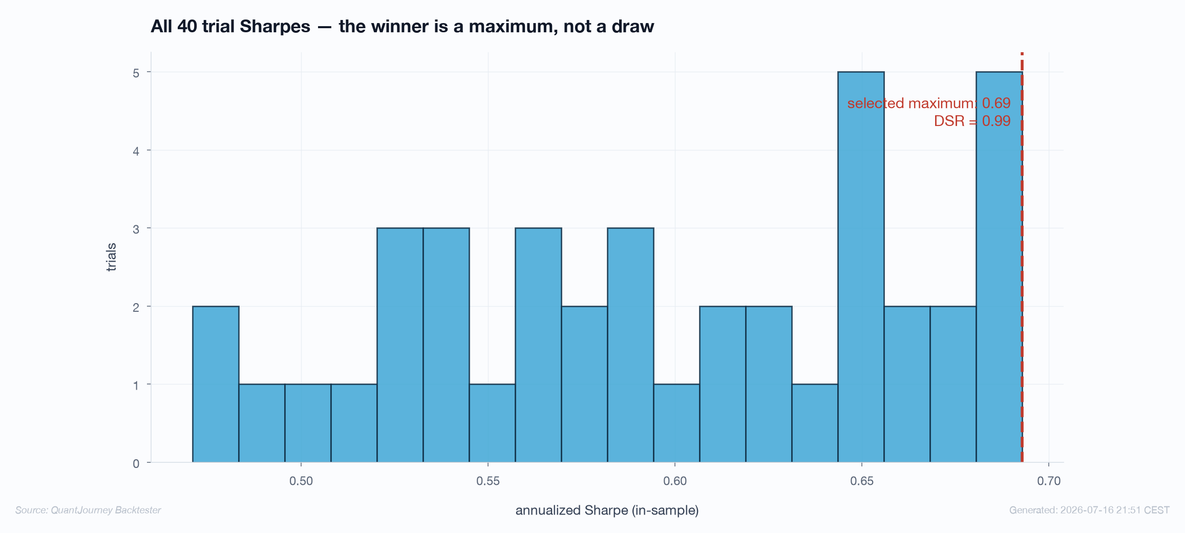
The Deflated Sharpe Ratio formalizes the question: it computes the expected maximum Sharpe that N effectively independent zero-skill trials would produce (given the trial count, the variance across trials, the sample length and the return distribution's skew and kurtosis), and reports the probability that the winner's true Sharpe exceeds that bar:
For this study: DSR = 0.99 — the winner clears the 40-trial luck bar decisively. Three structural reasons, worth internalizing because they generalize: the sample is long (19 years — T in the denominator of everything), the trial count is modest (40, not 4,000), and the surface is a plateau rather than a spike — the median trial (0.60) is respectable on its own, so selection added little. Compare the shipped thresholds: DSR ≥ 0.95 robust, 0.80–0.95 marginal, below 0.80 likely a false positive. A DSR of 0.55 with the same headline Sharpe would have meant "the search manufactured this" — same tear sheet, opposite verdict. The full formula and its inputs live in the statistical validation guide.
In the DSR formula N is the effective number of independent trials, not automatically the raw count of highly
correlated Optuna variants. The engine reports the finite completed count used to estimate trial variance and
accepts dsr_effective_n_trials; leaving it unset uses the raw completed count conservatively.
Pruned, failed and earlier "quick checks" still belong in the audit, and repeatedly resetting the study until
a metric passes remains undisclosed selection.
Read the study, not the winner
The trial table is research data. Five minutes of reading it distinguishes a defensible optimum from a lucky row.
# The study is research data - keep all of it, not just the winner.
df = result.all_results          # one row per trial

df.nlargest(5, "objective")      # is the top a plateau or a lone spike?
df["objective"].median()         # 0.60 here - the field, not the winner
df[["fast", "slow"]].describe()  # are winners piling up at a bound?

# Trials that died are data too:
# state == PRUNED  -> stopped early by the median rule (cheap negatives)
# state == FAIL    -> exceptions; investigate, never silently drop
# value == -999 -> constraint violations (should be ~0 with TPE)| Diagnostic | This study | What would worry us |
|---|---|---|
| Winner vs median trial | 0.69 vs 0.60 — shallow tail | Winner far beyond every other trial |
| Neighborhood of the winner | Dense cluster 0.65–0.69 around (40–55, 135–160) | Isolated spike; neighbors mediocre |
| Boundary pile-up | Winners interior to both ranges | Winners hugging a bound — the space truncates the surface |
| Convergence curve | Flat after trial 33 | Still climbing at budget end — search unfinished |
| Waste | 0 constraint violations (TPE) | Large pruned/failed fraction — dead space or broken objective |
The honest endgame: nest the search in the folds
A full-period search followed by a walk-forward of the winner is still not an OOS claim — the parameters saw every fold before the validation began. The engine closes that gap natively.
Pass the optimizer into the walk-forward engine and the search re-runs inside each fold's training window; the fold's winner is frozen and scored on that fold's held-out window, which nothing in the search ever touched. This is also what unlocks the two statistics the walk-forward guide reports as honestly unavailable without an optimizer: the DSR-style diagnostic pools finite per-fold trial values and labels that multi-fold extension explicitly, while the rolling top-K rank diagnostic re-runs each fold's top-K trials on the OOS window to see how often the in-sample favorite falls below the subset midpoint. That diagnostic is useful, but it is not canonical CSCV PBO because it does not use the complete N-configuration matrix or symmetric CSCV splits:
from backtester.walkforward import WalkForwardConfig, WalkForwardEngine

# The honest pattern: search runs INSIDE each fold's training window,
# the winner is frozen, and only then scored on that fold's OOS window.
config = WalkForwardConfig(
    scheme="rolling",
    train_months=24, test_months=6, step_months=6,
    purge_days=5, extra_pre_oos_purge_pct=0.01,
    compute_deflated_sharpe=True,   # explicitly labelled pooled WF DSR-style
    dsr_effective_n_trials=None,    # raw completed count if dependence is unknown
    compute_rank_stability=True,
    rank_stability_trials=8,        # rolling top-K diagnostic, not CSCV PBO
    seed=42,
)

engine = WalkForwardEngine(
    config=config,
    backtester_factory=factory,     # date-bounded strategy per fold
    optimizer=optimizer,            # the search, nested per fold
)
result = await engine.run_async(strategy.portfolio_data)

result.oos_sharpe        # composite of fold winners, scored out-of-sample
result.deflated_sharpe, result.deflated_sharpe_method
# pooled finite objectives across folds; not canonical single-population DSR
result.dsr_raw_completed_trials, result.dsr_effective_trials
result.walk_forward_top_k_rank_failure_rate  # descriptive, not CSCV PBO
For calibration, the cheap-but-weaker variant we ran here — full-period search, then slice-mode walk-forward of the frozen winner — produced OOS Sharpe 0.665, overfit ratio 0.70, efficiency 1.14 for (52, 141), against 0.513 for the untuned (50, 200) baseline. Encouraging, and correctly labeled: the tuning improved the sliced OOS numbers, but only the nested run above earns the sentence "the search process itself generalizes". Budget accordingly: nested cost is roughly n_folds × n_trials backtests — this is exactly where pruning and the engine's fold checkpointing pay for themselves.
Run it
# Optuna ships as an optional extra
pip install "quantjourney-bt[wf]"

# The published TPE + walk-forward example (30 trials, sector ETFs)
./strategy.sh example_wf_05_optuna_tpe_optimization

# Grid-search reference for small spaces
./strategy.sh example_wf_04_grid_search_optimization
A defensible optimization workflow
Bound the space by the hypothesis
Every parameter maps to an economic or implementation choice with a plausible domain. "Or maybe 2 days" is a fishing expedition, and it inflates N.
Freeze the objective before searching
Score, costs, degenerate-trial handling and penalties are part of the strategy specification — decided before the first trial, never adjusted to help.
Seed it and log everything
seed=42makes the search replayable;result.all_resultskeeps completed, pruned and failed trials so the research history and any effective-N assumption can be audited.Read the study before the winner
Plateau beats peak. Check the winner's neighborhood, boundary pile-ups and the convergence curve before quoting best_params anywhere.
Document the DSR trial assumption
Archive the raw finite completed count and the effective N used for dependence. If you searched repeatedly, disclose the full selection history rather than resetting it.
Nest the search for the OOS claim
WalkForwardEngine(optimizer=…)withrank_stability_trials=K— search inside training, freeze, score on the fold's OOS, and report the top-K metric by its non-CSCV name.
We do independent validation engagements — permutation tests, walk-forward, Deflated Sharpe and rank stability on your code or track record, delivered as a signed, reproducible report.
References
- Bergstra, J., Bardenet, R., Bengio, Y. & Kégl, B. (2011). Algorithms for Hyper-Parameter Optimization. NeurIPS — the TPE algorithm.
- Bergstra, J. & Bengio, Y. (2012). Random Search for Hyper-Parameter Optimization. JMLR 13 — why random beats grid in high dimensions.
- Akiba, T., Sano, S., Yanase, T., Ohta, T. & Koyama, M. (2019). Optuna: A Next-generation Hyperparameter Optimization Framework. KDD.
- Bailey, D. H. & López de Prado, M. (2014). The Deflated Sharpe Ratio. Journal of Portfolio Management 40(5) — the winner-vs-N correction.
- Bailey, D. H., Borwein, J., López de Prado, M. & Zhu, Q. J. (2017). The Probability of Backtest Overfitting. Journal of Computational Finance 20(4) — canonical CSCV PBO, which is distinct from the rolling top-K diagnostic above.
- White, H. (2000). A Reality Check for Data Snooping. Econometrica 68(5) — the original formalization of search-inflated performance.