Related is not revertible
Pairs trading is the cleanest laboratory in quantitative finance: one economic hypothesis (this spread mean-reverts), one state machine, two legs. It is also where wishful thinking hides best, because almost any two related instruments look like a pair. This guide builds the machinery — spread construction, hedge ratios, the z-score state machine — then runs it honestly on a pair that looks perfect and measurably is not, and shows the one-line diagnostic that would have told you first.
What a pairs backtest actually tests
The thesis is conditional and precise: this particular definition of the spread between A and B reverts to this particular definition of its mean, fast enough to beat costs. Nothing less specific is testable.
That precision is the point of the exercise. "KO and PEP move together" is a correlation observation — cheap, common and not a strategy. The tradeable claim is stronger: some combination of the two prices is stationary — it has a level it keeps coming back to — and deviations from that level are large and frequent enough to pay the round trips. Correlated returns do not imply any of this: two assets can be 0.9-correlated daily while their price ratio drifts forever (they co-move but re-scale). The statistical name for the property you actually need is cointegration, and the operational quantity that summarizes it for a trader is the spread's half-life of mean reversion — both measurable before a single backtest runs.
Scan 100 tickers for "good pairs" and you evaluate ~5,000 candidates — the best-looking spread of five thousand is spectacular by construction, cointegration tests included. Pair selection is a search process like any other: it needs the multiple-testing corrections (Romano–Wolf across the candidate family) and out-of-sample confirmation, or it needs to be replaced by a pre-declared economic argument, which is what the engine's examples do (KO/PEP, EWA/EWC — chosen for the economics, not mined from the data).
Constructing the spread
Two specifications ship with the engine; they differ in exactly one decision — whether the relationship between the legs is fixed or estimated.
The fixed log-ratio (example W13) assumes the pair moves 1:1 in log space — the simplest possible relationship, with no fitted hedge coefficient. It is an easy-to-reproduce baseline whose dominant model risk is long-run relative drift between the legs; pair selection, z-score settings, execution, borrow and financing risks still remain. The rolling hedge ratio (example W14) estimates the relationship from a trailing window by OLS:
# example_weights_14: the spread adapts, the sizing does not.
la, lb = np.log(close[a]), np.log(close[b])

beta = la.rolling(60).cov(lb) / lb.rolling(60).var()   # strictly trailing
spread = la - beta * lb
z = (spread - spread.rolling(60).mean()) / spread.rolling(60).std()

# beta changes WHICH series is normalized - the legs stay +/-0.5.
# A beta-SIZED book (w_B = -beta * w_A) is a different strategy with
# different gross exposure; normalize it explicitly if you build one.
The adaptive spread tracks a changing relationship — at the price of estimation risk (β is one more trailing window that can lag a break) and a subtlety the code comment above spells out: in W14 the estimated β changes the series being normalized, not the position sizes. The legs stay ±0.5. A book that sizes leg B at −β per unit of A is a different, leverage-varying strategy; if you want it, build it deliberately with explicit gross-exposure normalization — do not let it emerge from a spread formula by accident.
| Decision | W13 — fixed ratio | W14 — rolling hedge |
|---|---|---|
| Spread model | log(A) − log(B) | log(A) − β₆₀·log(B) |
| Estimated parameters | None | Rolling β (strictly trailing) |
| Fails when… | The 1:1 relation drifts | The relation breaks faster than 60 bars |
| Normalization | 60-bar rolling z-score, both examples | |
| Sizing | ±0.5 per leg — gross 1.0, net ≈ 0 | |
The z-score state machine
Entry and exit thresholds do not generate isolated signals — they drive a persistent position state. The asymmetry between them (enter at 2, exit at 0.5) is what prevents thrashing at the boundary.
class PairsRatioZScore(Backtester):
    """Market-neutral pair on a log-ratio z-score (example_weights_13)."""

    LOOKBACK = 60
    ENTRY = 2.0
    EXIT = 0.5

    def _compute_signals(self) -> pd.DataFrame:
        close = self.instruments_data.get_feature("adj_close")
        a, b = self.instruments[0], self.instruments[1]
        spread = np.log(close[a]) - np.log(close[b])
        z = (spread - spread.rolling(self.LOOKBACK).mean()) \
            / spread.rolling(self.LOOKBACK).std()

        signals = pd.DataFrame(0.0, index=close.index, columns=close.columns)
        state = 0            # +1 = long A / short B, -1 = short A / long B
        for i, zi in enumerate(z):
            if pd.isna(zi):
                state = 0                    # warm-up: flat, honestly
            elif state == 0:
                if zi > self.ENTRY:
                    state = -1               # A rich vs B -> short A, long B
                elif zi < -self.ENTRY:
                    state = 1                # A cheap vs B -> long A, short B
            elif abs(zi) < self.EXIT:
                state = 0                    # reverted -> unwind
            signals.iloc[i] = [state, -state]
        return signals

    def _compute_weights(self) -> pd.DataFrame:
return self.signals * 0.5 # +/-0.5 per leg: gross 1.0, net ~0Two engine disciplines do quiet work here. The warm-up rows are honest zeros (the workflow guide's trap 2), and the state machine's decisions are shifted one bar by the engine's accounting — the z-score computed from tonight's closes earns tomorrow's spread move, never tonight's. Every rolling statistic in both examples is strictly trailing for the same reason: a sizing or signal layer that peeks is look-ahead wearing a costume.
The diagnostic that comes before the backtest
One regression tells you whether the spread reverts on a horizon your window can trade — before you spend a single backtest on it.
Model the spread as an AR(1) in changes: regress today's spread change on yesterday's spread level. A negative coefficient means deviations pull back toward the mean, and its size converts directly into the half-life — the expected time for a deviation to close half the gap:
# The diagnostic that comes BEFORE any backtest: does this spread
# actually mean-revert on a horizon your window can trade?

spread = np.log(close["TLT"]) - np.log(close["IEF"])

ds = spread.diff().dropna()                  # AR(1) on spread changes
s_lag = spread.shift(1).dropna().loc[ds.index]
b = np.polyfit(s_lag - s_lag.mean(), ds, 1)[0]

half_life = -np.log(2) / np.log(1 + b)       # b must be negative
print(f"half-life: {half_life:.0f} trading days")
# TLT/IEF, 2007-2026:  473 days

# Rule of thumb: the z-score LOOKBACK should live on the same scale
# as the half-life. A 60-day window on a 473-day spread does not
# measure reversion - it measures noise around a drifting level.
The rule of thumb it enables: the z-score lookback and the half-life must live on the same scale. A 60-day window on a 20–60-day half-life spread measures genuine stretch and snap-back. The same window on a 473-day half-life spread measures noise around a level that migrates slower than the window can see — every "entry" is a bet that a random wiggle reverts, and the position's fate is decided by the drift, not the spread.
A measured example: TLT/IEF, and why it loses
Long and intermediate Treasuries: same issuer, same rate factor, correlation ~0.9. The most plausible-looking pair in the ETF universe — and the diagnostic above already said no.
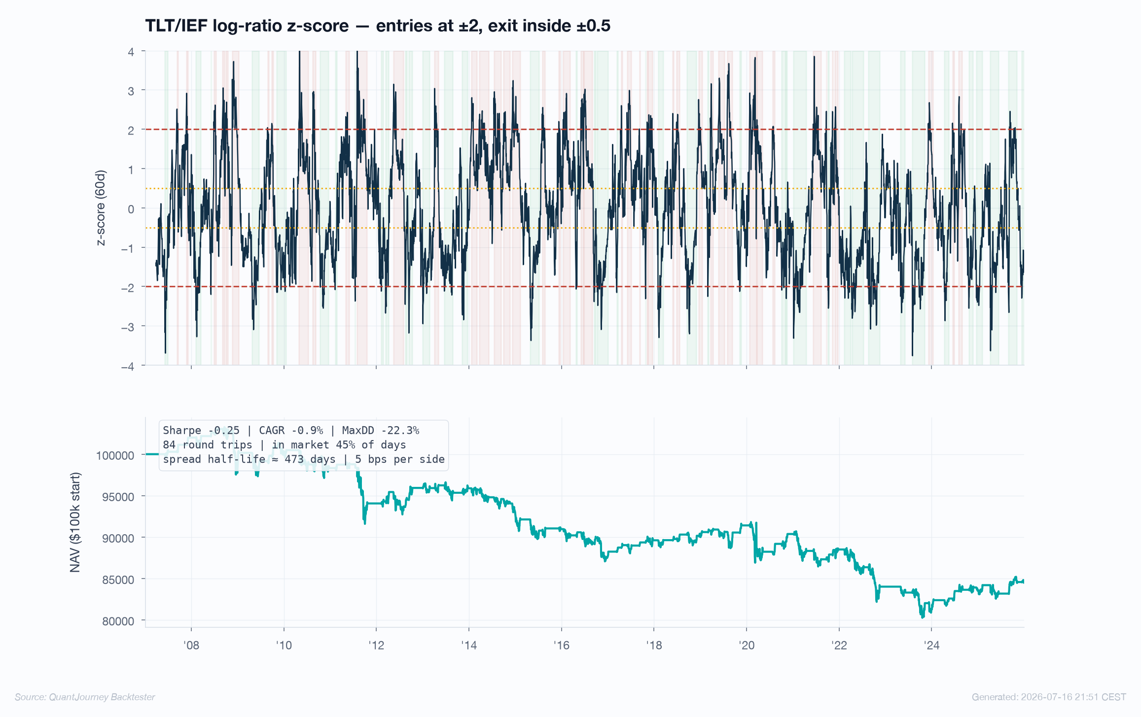
We ran the W13 machinery exactly as shipped — 60-day z-score, ±2 entry, 0.5 exit, daily rebalance, 5 bps per side — on TLT/IEF over 2007–2026, on the engine's fast-weights path. The half-life of the log-ratio is 473 trading days: the spread is dominated by slow, persistent moves in the yield curve's shape (duration exposure differs by design), not by a stationary relationship. The backtest agrees with the diagnostic:
| Metric | Value | Reading |
|---|---|---|
| Sharpe | −0.25 | The machinery traded noise, net of costs |
| CAGR | −0.88% | A slow bleed, not a blow-up |
| Max drawdown | −22.3% | 19 years of compounding small losses |
| Ann. volatility | 3.3% | "Market neutral" ≠ safe — just quiet |
| Round trips | 84 | ~4.4 per year, in market 45% of days |
| Turnover / costs | 9.5× · $8,268 | 0.47%/yr of drag on a 3.3%-vol book |
| Spread half-life | 473 days | vs a 60-day window — the mismatch that decided everything |
pair = PairsRatioZScore(
    api_key=os.environ.get("QJ_API_KEY"),
    strategy_name="Pairs_TLT_IEF",
    strategy_type="Market Neutral",
    initial_capital=100_000,
    instruments=["TLT", "IEF"],
    backtest_period={"start": "2007-01-03", "end": "2026-01-01"},
    benchmark_symbol="SPY",
    source="yfinance",
    execution_mode="weights",
    rebalance_policy=RebalancePolicy(frequency="D"),
    weight_cost_model=FixedBpsWeightCostModel(total_bps=5.0),
    indicators_config=[],
)
await pair.run_strategy()
pair.print_summary()
Why publish a losing run? Because this is the most common pairs-trading failure in the wild, and it never looks like a failure in advance: high correlation, an obvious economic link, a z-score that generates confident entries — every surface indicator says trade it. The half-life regression is the one-line test that separates this pair from a tradeable one, and it costs nothing. The shipped KO/PEP and EWA/EWC examples pass the same sanity scale; TLT/IEF is the control group.
Dollar-neutral is not risk-neutral
±0.5 per leg targets near-zero net dollar exposure. Everything else — beta, duration, factor and currency exposure — must be checked, not assumed.
The TLT/IEF book above is dollar-neutral and still carries a large structural exposure: long one duration, short another, it is a leveraged bet on the yield curve's slope — which is precisely the slow factor that dominated its spread. Equity pairs inherit sector and market beta whenever the legs' betas differ; country pairs (EWA/EWC) carry currency. The portfolio reports make this visible — per-leg realized weights, gross and net exposure, and the benchmark-relative rolling beta chart — and reading them is part of the strategy, because a "market-neutral" label on a factor bet is how quiet books produce loud surprises.
Costs, borrow and capacity
A mean-reversion book pays costs on every round trip and holds two legs while it waits. Small frictions dominate small edges.
The measured run already shows the arithmetic: 9.5× annual turnover at 5 bps costs 47 bps a year — on a book whose gross volatility is 3.3%, that is a seventh of the risk budget spent on friction before any edge is earned (the costs guide develops the full turnover-drag machinery). Two costs the engine's research baseline deliberately does not model deserve explicit mention in any pairs write-up: short borrow — availability, fees and recall risk on the short leg, which for hard-to-borrow names can exceed the spread edge outright — and leg execution risk — the two legs do not fill simultaneously in practice, and a fast-moving spread charges the gap to you. Both belong in the orders-path stress test before any live deployment.
Validating a pairs strategy
Everything in the site's validation toolkit applies, with one pairs-specific emphasis: the selection of the pair is part of the process being tested.
The MCPT signal-timing test asks whether the state machine's
timing beats circular-shift null paths of itself; bar-permutation kills the spread's temporal structure and demands the
edge die with it (the pure weight_fn both examples use makes them directly testable). If
parameters were tuned — lookback, entry, exit — the search belongs
inside walk-forward folds with DSR and explicitly labeled rank stability on the record. And if
the pair itself was screened from a universe, the candidate family goes through Romano–Wolf: the best of 5,000
spreads must survive being the best of 5,000, not just beat its own shuffles.
Run both specifications
# Fixed 1:1 log-ratio, KO / PEP (consumer staples)
./strategy.sh example_weights_13_pairs_ratio_zscore

# Rolling OLS spread, EWA / EWC (country ETFs)
./strategy.sh example_weights_14_pairs_hedge_ratio
The pairs checklist
Declare the pair before touching data
An economic argument for the relationship, written first — or a mined selection corrected for the full family it was mined from.
Measure the half-life first
One AR(1) regression. If it is several times your intended z-window, stop — the machinery will trade noise around a drift, as TLT/IEF demonstrates.
Match the window to the physics
Lookback on the half-life's scale; entry/exit asymmetric (2.0 / 0.5) so the state machine does not thrash at the boundary.
Audit both legs, not the combined NAV
Per-leg weights, gross and net exposure, rolling beta vs benchmark — dollar-neutral books hide factor bets in plain sight.
Stress the frictions the baseline omits
Borrow fees on the short leg, leg-fill asynchrony, and the cost ladder — a 3%-vol book has no room for 1% of friction.
Validate like any other strategy
MCPT on the final configuration, walk-forward for tuned parameters, Romano–Wolf when the pair came from a screen.
We do independent validation engagements — permutation tests, walk-forward, Deflated Sharpe and rank stability on your code or track record, delivered as a signed, reproducible report.
References
- Gatev, E., Goetzmann, W. & Rouwenhorst, K. G. (2006). Pairs Trading: Performance of a Relative-Value Arbitrage Rule. Review of Financial Studies 19(3) — the canonical empirical study.
- Engle, R. F. & Granger, C. W. J. (1987). Co-integration and Error Correction. Econometrica 55(2) — why correlation is not the property you need.
- Avellaneda, M. & Lee, J.-H. (2010). Statistical Arbitrage in the US Equities Market. Quantitative Finance 10(7) — OU modeling of spreads at scale.
- Vidyamurthy, G. (2004). Pairs Trading: Quantitative Methods and Analysis. Wiley.
- Chan, E. (2013). Algorithmic Trading: Winning Strategies and Their Rationale. Wiley, ch. 2–3 — the half-life heuristic this guide operationalizes.
- Do, B. & Faff, R. (2010). Does Simple Pairs Trading Still Work? Financial Analysts Journal 66(4) — the decay of the classic rule after costs.