From idea to strategy
Most strategies do not fail in production. They fail months earlier — in a hypothesis that was never written down, a look-ahead bug that flattered every iteration, a cost assumption that was never stressed, or a p-value that was never computed. This guide walks the full pipeline in order: what to do at each stage, what to look at in the code, which numbers to demand before moving on — and where each gate lives in the engine. The worked examples run on real data, and the validation example fails its own gate. That is the point.
A strategy is a hypothesis, not a script
The difference between research and curve-fitting is not talent. It is the order of operations.
A trading strategy is a falsifiable claim about how markets misprice something, wearing enough engineering to be executed. The claim comes first; the code is its experiment. When the order is reversed — write a script, tweak it until the equity curve looks right, then invent a story — every downstream tool still runs, every report still renders, and every number is still meaningless. No statistical test can rescue a process that optimized first and asked questions later, because by then the data has already been spent.
The pipeline below is the order of operations we use for every strategy that ships into the engine's example suite. Each stage has a concrete deliverable and an exit gate — a number or an artifact that must exist before the next stage is allowed to start. The stages are cheap early and expensive late, which is exactly why the order matters: a hypothesis is falsified in an afternoon, a production false positive costs months of drawdown before it confesses.
| Stage | Deliverable | Exit gate | Engine surface |
|---|---|---|---|
| 0 · Hypothesis | Written economic claim | Falsifiable + names who loses | — |
| 1 · Data & universe | Universe + period + data contract | Covers ≥ 2 hostile regimes | instruments=, backtest_period=, strict fetch |
| 2 · Prototype | Simplest runnable strategy | Behaves as hypothesized before tuning | Backtester subclass, weights mode |
| 3 · Code audit | The four traps checked | Pure, shifted, warm-up-honest, costed | _compute_signals / _compute_weights |
| 4 · Cost stress | Cost ladder table | Alive at 2× realistic costs | FixedBpsWeightCostModel |
| 5 · Optimization | Search log, every trial kept | Pre-committed DSR/rank-stability policy | WalkForwardEngine + Optuna |
| 6 · Statistical gates | mcpt.json verdicts | MCPT p < 0.05, Romano–Wolf survives | backtester.validation |
| 7 · Decision | Deployment note + archive | All gates green, kill criteria written | Run archive + fingerprints |
Running the statistical gates after iterating freely on the full sample tests a different thing than you think: it tests the best of everything you tried, with the selection bias baked in. Stage 5 exists to make the search itself auditable; stage 6 quantifies what survives it. Skip the bookkeeping and the same tools return flattering, wrong answers.
Stage 0 — write the hypothesis before the code
Five lines of text, written before the first import, are the cheapest risk management you will ever do.
An economic hypothesis says why a strategy should make money: which risk premium it harvests, which behavioral bias it exploits, or which structural constraint it arbitrages — and, crucially, who is on the other side of the trade and why they accept losing it. This is not academic ritual. The hypothesis is what tells you, months later, whether the edge decayed (the mechanism disappeared — retire it) or merely drew down (the mechanism is intact — hold). Without it, every drawdown becomes an unanswerable question.
# hypothesis.md - written BEFORE any code
#
# CLAIM      Liquid asset-class ETFs above their long-term trend retain
#            positive directional persistence over the next month.
# WHY        Slow information diffusion, behavioral herding and gradual
#            institutional de-risking create medium-term trend persistence.
# WHO LOSES  Investors forced to rebalance late or hold static exposure
#            through persistent market regimes.
# DIES WHEN  Crowding compresses the premium; turnover cost exceeds it.
# TESTABLE   The SMA(50/200) long/cash basket beats its circular-shift timing null
#            (MCPT p < 0.05) net of 5 bps, and survives walk-forward OOS.
#
# If you cannot fill in WHO LOSES, you are describing a pattern,
# not an edge. Patterns without a counterparty rarely survive costs.
The last line matters most: the hypothesis commits, in advance, to the test that would falsify it. That commitment is what separates a research process from a narrative generator. It also fixes the metric, the cost assumption and the significance threshold before any of them can be chosen to flatter the result.
Stage 1 — data and universe honesty
Every backtest is a claim conditional on its data. Most inflated backtests are data problems wearing a strategy costume.
Three questions decide whether the data can support the claim. Does the universe contain the losers?
A universe built from today's index members silently deletes everything that died on the way — and dead companies
are where short signals and risk lessons live. Broad ETFs reduce constituent-level survivorship work for asset-class
strategies, but they do not eliminate ex-post fund-selection bias; single-name universes need point-in-time membership.
Are corporate actions handled once, in the data layer?
The engine's adj_close feature reinvests dividends and absorbs splits consistently; strategy code that
re-adjusts prices is a bug factory. Does the period contain at least two regimes that should hurt?
A trend strategy tested on 2009–2021 has never met 2022; a carry strategy that starts in 2010 has never met 2008.
UNIVERSE = ["SPY", "EFA", "EEM", "TLT", "IEF", "GLD", "DBC", "VNQ"]
PERIOD   = {"start": "2007-01-03", "end": "2026-01-01"}

# Why these choices survive scrutiny:
#  - ETFs reduce single-stock constituent-survivorship problems, but do
#    not remove ex-post universe-selection bias. Every selected fund
#    existed throughout this window; no constituent-history reconstruction
#    is required for this example, and no selected fund delists in-sample.
#  - adj_close everywhere: dividends reinvested, splits handled once,
#    consistently, in the data layer - not in strategy code.
#  - 2007 start: the sample contains 2008, 2020 AND 2022 - three
#    different ways to lose money. A backtest that starts in 2009
#    has never seen its strategy's worst regime.
#  - strict fetch: the engine raises on missing instruments instead of
#    silently shrinking the universe (allow_partial_data=False default).
The engine enforces the contract at fetch time: requested instruments must arrive (no silent universe shrinkage),
close or adjusted close must exist, and missing observations stay NaN — a date with no price is an
unknowable, not a zero. Weight-mode accounting poisons dates where a held instrument has no return rather than
booking a phantom flat day. Fabricated zeros average into every statistic downstream; honest NaN refuses to.
Stage 2 — the simplest version that could work
The prototype's job is not to be good. Its job is to be simple enough that nothing can hide in it.
One signal, equal weights, monthly rebalance, default costs. No optimization, no sizing overlays, no filters — every one of those is a knob you will later have to defend, so the baseline earns credibility by having none. The complete strategy is under forty lines against the engine:
import asyncio
import os
import pandas as pd

from backtester import Backtester
from backtester.portfolio.rebalance import RebalancePolicy


class TrendBasket(Backtester):
    """SMA(50/200) trend basket - the simplest version that could work."""

    def _compute_signals(self) -> pd.DataFrame:
        fast = self.instruments_data.get_feature("SMA_50_close")
        slow = self.instruments_data.get_feature("SMA_200_close")
        valid = fast.notna() & slow.notna()
        return (fast > slow).astype(float).where(valid, 0.0)

    def _compute_weights(self) -> pd.DataFrame:
        active = self.signals == 1.0
        counts = active.sum(axis=1)
        return active.div(counts.where(counts > 0), axis=0).fillna(0.0)


async def main() -> None:
    strategy = TrendBasket(
        api_key=os.environ.get("QJ_API_KEY"),
        strategy_name="TrendBasket_v0",
        strategy_type="Long / Cash",
        initial_capital=100_000,
        instruments=["SPY", "EFA", "EEM", "TLT", "IEF", "GLD", "DBC", "VNQ"],
        backtest_period={"start": "2007-01-03", "end": "2026-01-01"},
        benchmark_symbol="SPY",
        source="yfinance",
        execution_mode="weights",
        rebalance_policy=RebalancePolicy(frequency="BME"),
        indicators_config=[
            {"function": "SMA", "price_cols": ["close"], "params": {"periods": [50, 200]}},
        ],
        save_text_reports=True,
        save_portfolio_plots=True,
    )
    await strategy.run_strategy()
    strategy.print_summary()


if __name__ == "__main__":
    asyncio.run(main())
Two structural choices in this template do quiet, load-bearing work. _compute_signals and
_compute_weights are separate stages: the signal says what looks attractive, the weights say
how much capital that conviction gets — keeping them apart is what lets you later swap the sizing scheme
without touching the signal (the sizing guide does exactly
that, on this exact strategy). And the strategy computes targets, not trades: the declarative
RebalancePolicy decides when targets become transactions, which is what makes trading frequency a
measurable dial instead of a side effect (the costs guide measures that
dial).
Run on the canonical eight-ETF universe, 2007–2026, at 5 bps per side, this baseline earns a 5.1% CAGR at 10.9% volatility — Sharpe 0.51, max drawdown −22.2%, engine-computed. Unremarkable, and exactly what stage 2 should produce: a number the hypothesis predicted would exist (trend following works in multi-asset baskets, modestly), measured before any knob was turned. If your prototype's Sharpe is already 2.0, do not celebrate — go directly to stage 3, because something is leaking.
Stage 3 — the four code traps that fake alpha
Many inflated backtests we inspect contain at least one of four recurring implementation failures. The list is not exhaustive — universe selection, stale prices, corporate actions, borrow constraints and fill assumptions belong in the surrounding data and execution audits. These four can all produce beautiful equity curves.
Trap 1 — look-ahead. The oldest and still the most common: scoring today's decision with today's return. The engine's accounting shifts target weights one bar — a decision made from information up to t earns the return from t to t+1, never the bar it was computed on:
# TRAP 1 - look-ahead. The engine shifts weights one bar for you:
# decide at t, earn r[t+1]. Reconstructing returns yourself?
# Keep the same discipline or your Sharpe is fiction.

held = weights.shift(1)                          # RIGHT: yesterday's decision
r_p = (held * instrument_returns).sum(axis=1)

r_wrong = (weights * instrument_returns).sum(axis=1)   # WRONG: trades on
                                                       # information from the
                                                       # bar being traded
One shifted index is routinely worth a full Sharpe point on daily momentum signals — which is why "shift discipline" is the first thing to check in any strategy whose numbers look too smooth.
Trap 2 — indicator warm-up. An SMA(200) does not exist for the first 200 bars. What your code does on those bars is a policy decision. An implicit comparison currently happens to produce zero, but an explicit validity mask makes the policy stable and auditable; forward-filling later gaps can trade on stale information:
# TRAP 2 - indicator warm-up. SMA(200) is NaN for 200 bars.
fast, slow = sma_50, sma_200

valid = fast.notna() & slow.notna()
signals = (fast > slow).astype(float).where(valid, 0.0)   # RIGHT: flat, honestly

signals_bad = (fast > slow).astype(float)          # FRAGILE: currently also gives
                                                   # zero because NaN comparisons
                                                   # are False, but hides the policy
signals_worse = (fast.ffill() > slow.ffill())      # RISKY for later data gaps: may
                                                   # trade on stale indicator values
Trap 3 — hidden global state. A weight function that touches anything precomputed on the real market cannot be honestly re-fit — not on walk-forward folds, not on permuted markets, not on tomorrow's data. Purity is not a style preference; it is what makes stage 6's market-rebuild specification (bar-permutation MCPT, which re-runs the strategy on synthetic markets) mathematically valid:
# TRAP 3 - hidden global state. Everything derives from what the
# function receives. This is also what makes bar-permutation MCPT
# (and any re-fit on synthetic data) valid later.

def weight_fn(prices: pd.DataFrame) -> pd.DataFrame:      # RIGHT: pure
    fast = prices.rolling(50).mean()
    slow = prices.rolling(200).mean()
    active = (fast > slow) & fast.notna() & slow.notna()
    return active.astype(float).div(active.sum(axis=1).clip(lower=1), axis=0)

SMA_CACHE = prices.rolling(50).mean()                     # WRONG: computed once
def weight_fn_bad(p: pd.DataFrame) -> pd.DataFrame:       # on the REAL market,
    return (SMA_CACHE > p.rolling(200).mean()).astype(float)  # smuggled into
                                                              # every re-fit
Trap 4 — costs at zero. Not a bug in the code, a bug in the defaults: every comparison, from the first prototype onward, should run with a nonzero cost assumption, because costs change rankings, not just levels — a faster variant can beat a slower one gross and lose to it net. The engine's weight-mode default is 1 bp; stage 4 stresses it properly.
That is the stage 3 exit gate: all four hold before any number from the prototype is quoted to anyone — including yourself.
Stage 4 — stress costs before tuning anything
Costs are among the assumptions most likely to be underestimated in research and to deteriorate with live execution or scale. Stress them first, so every later decision is made net.
The mechanics are one line of config — the same strategy, run across a ladder of cost assumptions:
from backtester.portfolio.weight_cost import FixedBpsWeightCostModel

# Same strategy, six cost assumptions - run the ladder BEFORE tuning.
for bps in [0, 1, 5, 10, 25, 50]:
    strategy = XSMomentum(
        ...,
        weight_cost_model=FixedBpsWeightCostModel(total_bps=bps),
    )
    await strategy.run_strategy()
In this model, total_bps is applied to each buy or sell notional. The table therefore reports the
configured rate per side; it is not silently doubling a round-trip input.
To make the sensitivity visible, this cost illustration uses a higher-turnover companion example: a 126-day cross-sectional momentum strategy (top 3 of the 8 ETFs, monthly rebalance, 2007–2026). It is not the stage 2 trend prototype; every row below is a full engine run of this companion strategy:
| Cost per side | CAGR | Sharpe | Max DD | Final NAV ($100k start) | Total costs paid |
|---|---|---|---|---|---|
| 0 bps (gross) | 10.89% | 0.879 | −20.1% | $712,374 | $0 |
| 1 bp | 10.83% | 0.875 | −20.1% | $704,873 | $3,321 |
| 5 bps | 10.58% | 0.857 | −20.2% | $675,646 | $16,180 |
| 10 bps | 10.27% | 0.835 | −20.3% | $640,805 | $31,328 |
| 25 bps | 9.36% | 0.768 | −20.7% | $546,661 | $71,155 |
| 50 bps | 7.84% | 0.656 | −22.2% | $419,370 | $121,778 |
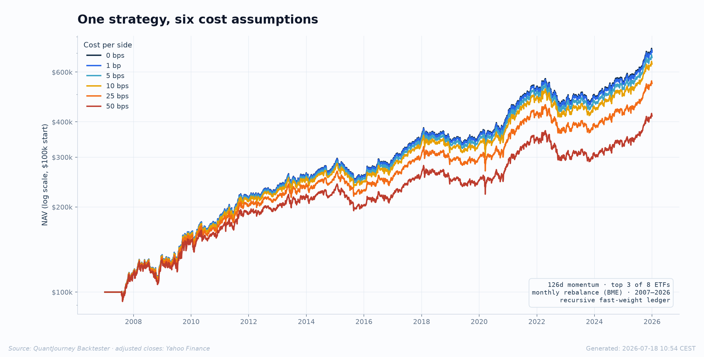
The decay is almost perfectly linear, and the slope is predictable from two numbers you already have — annual turnover and volatility:
This strategy turns over ≈ 5.58× NAV per year at 12.7% volatility, so each basis point of per-side cost predicts ≈ 0.0044 of Sharpe decay at first order. The engine-measured ladder closely tracks that estimate; the costs guide overlays them and documents the recursive accounting identity. The stage 4 rule of thumb: estimate your realistic all-in cost, then demand the strategy stays deployable at twice that number. If 10 bps kills it, it is not a strategy — it is a donation to your broker with extra steps.
Stage 5 — optimize with the search on the record
Optimization is not the enemy. Undocumented optimization is. The difference is whether N — the number of things you tried — is written down.
Every trial you evaluate raises the bar the winner must clear, whether or not you remember trying it. For independent Gaussian zero-skill results, the expected maximum grows asymptotically like √(2 ln N). This leading-order expression overstates the finite-sample expectation, but correctly shows how selection raises the hurdle as the search expands:
The defense is bookkeeping, and the engine does it for you when the search runs inside the walk-forward: every
Optuna trial — including pruned and failed ones — is logged. The walk-forward Sharpe-selection diagnostic uses
finite completed objectives pooled across folds and a documented effective-number-of-independent-trials
assumption; because those objectives come from different training windows, the engine labels it
pooled_walk_forward_dsr_style, not canonical single-population DSR. The second metric re-runs the top
K in-sample trials on each rolling OOS fold and reports a descriptive rank failure rate; it is not canonical CSCV PBO:
from backtester.walkforward import WalkForwardConfig, WalkForwardEngine

config = WalkForwardConfig(
    scheme="rolling",
    train_months=24, test_months=6, step_months=6,
    purge_days=5, extra_pre_oos_purge_pct=0.01,
    compute_deflated_sharpe=True,
    dsr_effective_n_trials=None,    # raw completed count if dependence is unknown
    compute_rank_stability=True,
    rank_stability_trials=8,        # rolling top-K diagnostic, not CSCV PBO
    seed=42,                        # the search itself is reproducible
)

engine = WalkForwardEngine(config=config,
                           backtester_factory=factory,
                           optimizer=optimizer)
result = engine.run(strategy.portfolio_data)

result.deflated_sharpe
result.deflated_sharpe_method  # pooled_walk_forward_dsr_style | probabilistic_sharpe_n1
result.dsr_raw_completed_trials, result.dsr_effective_trials
result.walk_forward_top_k_rank_failure_rate
Any gate on the pooled DSR-style extension is a pre-committed workflow convention, not a canonical threshold. The rolling top-K failure rate likewise has no canonical CSCV threshold: report its K, fold geometry and value as a sensitivity diagnostic. Canonical PBO would require the complete configuration matrix and symmetric CSCV combinations.
Three habits keep the search honest. Bound the space by the hypothesis — a momentum lookback grid of 3–12 months is a hypothesis refinement; adding "…or maybe 2 days" is a fishing expedition. Never re-tune to pass a gate — if stage 6 rejects the tuned strategy and you adjust parameters until it passes, the p-value you finally report is the best of many, which is precisely the bias the gate existed to catch. Prefer plateaus to peaks — a parameter whose neighbors all work is a property of the market; an isolated spike is a property of the sample. The full treatment — search spaces, objectives, trial diagnostics — is in the Optuna guide.
Stage 6 — the statistical gates
Everything so far produced a candidate. This stage asks the only question that matters: is the number distinguishable from luck?
The reference test is the Monte Carlo Permutation Test: move the strategy's decision path against the same market,
re-score each null path through the same accounting, and read where the real strategy lands. The primary
signal_timing specification is weight_null="circular_shift": one non-zero shift moves the
whole weight matrix, preserving its cyclic holding periods, transitions and nearly all turnover while breaking
calendar alignment. Full row permutation also destroys persistence and is an aggressive sensitivity test;
bar permutation rebuilds the strategy on synthetic markets and tests a different null. The rank calculation
requires no Gaussian return assumption, but validity still depends on the chosen transformation:
Here is the gate run on a separate validation example from the same trend-rule family in the engine suite — an SMA(50/200) rule on nine sector ETFs, 26 years of daily data, seed pinned, one function call. It is intentionally distinct from the eight-asset prototype above and demonstrates the gate rather than extending that backtest:
from backtester.validation import MCPTConfig, MCPTRunner

config = MCPTConfig(mode="signal_timing", n_permutations=1000,
                    metric="sharpe", weight_null="circular_shift", seed=42)
result = MCPTRunner(config).run_portfolio(strategy.portfolio_data)

print(result.summary())
result.save(f"reports/{strategy.strategy_name}/validation")

# Our own demo strategy, scored honestly:
#   Observed sharpe (annualized):  0.61
#   Null median (annualized):      0.52
#   p-value:                       0.135
#   Verdict: consistent with luck (p >= 0.10)
#
# A 26-year Sharpe of 0.61 - and it does NOT clear its own shifted
# null paths. That is the gate doing its job.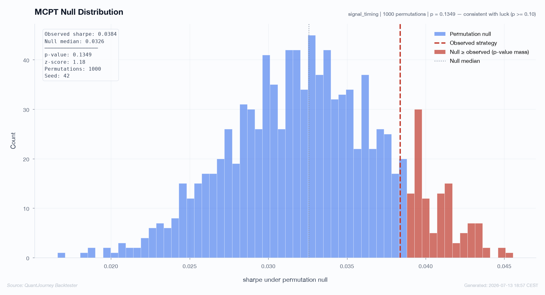
Sit with the result for a moment, because it is the most instructive number in this guide. A strategy with a 26-year track record and an annualized Sharpe of 0.61 fails to beat its circular-shift null paths. They retain the same fixed market, cyclic position sequence, holding periods and nearly all turnover, but lose the original calendar alignment. The median null earns an annualized 0.52. The observed timing contribution is positive but too weak to distinguish reliably from that null at the 5% level. A tear sheet would never tell you this; the tear sheet looks great.
What stage 6 does not license is quietly returning to stage 5 to fix the verdict. A failed gate sends you back to stage 0 with information: either the hypothesis is wrong, or the expression of it is too weak, or the data cannot support a verdict at this sample size. All three are findings. "Iterate until significant" is not — it is the manufacture of a false discovery, one honest-looking p-value at a time. The full machinery — the three permutation modes, Romano–Wolf for candidate families, DSR, rolling rank stability and canonical PBO context — is the statistical validation guide; the deployment thresholds live there too.
Stage 7 — the deployment decision
The last stage is a piece of writing, not a piece of code: the note that future-you will read during the first real drawdown.
By now the evidence exists as artifacts — every run archived with its config, data fingerprint and seed, every verdict in a machine-readable file. The deployment note assembles them and adds the one thing no engine can compute: the pre-committed conditions under which you will turn the strategy off.
reports/TrendBasket_v0/
├── run_metadata.json        # config, dataset id, package versions, seed
├── performance_report.txt   # the full text report
├── portfolio_data.pkl       # NAV, weights, returns - the evidence
├── instruments_data.pkl     # the exact market data the run saw
├── plots/                   # 39 institutional charts
└── validation/
    ├── mcpt.json            # p-value, z-score, verdict, SHA-256 fingerprint
    ├── mcpt_null_distribution.png
    └── mcpt_equity_fan.png

# Every claim in your research note should trace to one of these files.
# If the archive cannot reproduce the number, the number does not exist.
All pre-committed gates green, on the record
Cost-stressed baseline, the workflow's documented DSR/rank-stability policy, MCPT threshold and walk-forward OOS requirement — each traceable to an archived artifact, none chosen after seeing the result.
Sizing decided by risk, not conviction
The capital the strategy gets is an output of the risk-budgeting layer, sized so its worst archived drawdown is survivable at the allocated weight.
Kill criteria written before day one
The drawdown, the tracking gap versus backtest, and the time horizon at which you stop — decided now, while you are still objective, not during the event.
The hypothesis rides along
Attached to the deployment note, so every future review asks "is the mechanism intact?" instead of "how do I feel about the equity curve?"
Eighteen months from now, someone — probably you — will ask why this strategy is trading and whether the live results match what was promised. The archive answers with evidence: the exact data, the exact config, the exact verdicts, each with a fingerprint. Research that cannot be replayed is not research; it is a memory of one.
What failure costs at each stage
The pipeline's economics in one table: the same flaw, caught later, costs orders of magnitude more.
| Flaw | Caught at stage… | Cost of catching it there |
|---|---|---|
| No real mechanism, just a pattern | 0 — hypothesis won't write | One afternoon |
| Universe missing the losers | 1 — data audit | A day of data work |
| Look-ahead in the signal | 3 — shift audit | One code review |
| Edge thinner than costs | 4 — cost ladder | Six engine runs |
| Winner is best-of-500 noise | 5 — DSR and rank-stability audit | Minutes, automatic |
| Timing indistinguishable from luck | 6 — MCPT | One function call |
| All of the above, undetected | Production | Months of drawdown + the capital + the trust |
Every row above the last one is a success story — the process converting a would-be production failure into a cheap, early "no". A research pipeline should reject most of what enters it. If everything you try reaches deployment, the pipeline is not validating; it is decorating.
We do independent validation engagements — permutation tests, walk-forward, Deflated Sharpe and rank stability on your code or track record, delivered as a signed, reproducible report.