Make the information boundary visible
A full-period backtest mixes discovery, tuning and evaluation into one number. Walk-forward splits history into repeated train/test boundaries so you can watch the only thing that matters: what the strategy does on data that had no influence on it. This guide covers the engine's two walk-forward modes and why they carry different evidentiary weight, fold geometry, pre-OOS purging, and the reading of the result object — all demonstrated on a real 34-fold run whose fold-level noise is exactly the lesson.
Why a single backtest is not enough
One historical path, scored once, cannot distinguish a strategy from a coincidence. Walk-forward manufactures the thing a single backtest lacks: repetition with a boundary.
The mechanism is chronological discipline. Take the full history, mark a training window and a test window that follows it, evaluate on the test window only, then step both windows forward and repeat. Everything the strategy is allowed to learn — parameters, scalers, universe choices — must come from the training side of each boundary; everything it is judged on sits strictly after. What you get is not one number but a population of out-of-sample episodes, and populations support questions a point estimate cannot: does performance persist, decay, or concentrate in one lucky regime?
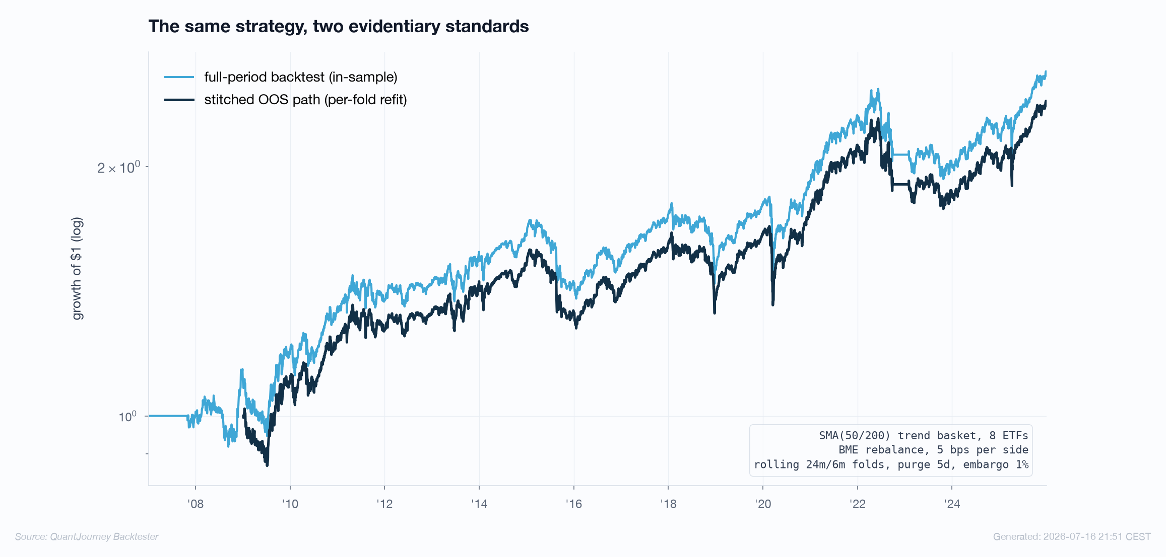
This guide's running example: the SMA(50/200) trend basket from the workflow guide — eight multi-asset ETFs, monthly rebalance, 5 bps per side, 2007–2026 — under a rolling 24-month train / 6-month test / 6-month step geometry with a 5-day purge plus a 1% pre-OOS extension. That yields 34 folds and, stitched together, 17 years of walk-forward OOS returns, conditional on the strategy and fold geometry having been specified before those folds were inspected. Every number and both charts below come from that run.
Leakage also enters through data revisions, survivorship in universe construction, features normalized on the full sample, overlapping labels, or parameters chosen after peeking at all folds. Fold geometry cannot repair an upstream process that already consumed the future — the code-trap audit comes first, walk-forward second.
Two modes, two classes of evidence
The engine deliberately exposes the distinction most tools blur: slicing a finished path is diagnostics; re-running the strategy inside each fold is evidence.
Slice diagnostics runs the strategy once over the full period and then cuts the finished portfolio path into train/test-shaped windows. It is fast — one backtest, then pure arithmetic — and it answers real questions: is performance concentrated in one era, does the OOS half of each fold look systematically worse than the IS half, how noisy are six-month episodes? What it cannot claim is out-of-sample discipline, because the single underlying run computed its indicators and weights on the whole history at once.
from backtester.walkforward import WalkForwardConfig, WalkForwardEngine

config = WalkForwardConfig(
    scheme="rolling",          # or "expanding" / "anchored"
    train_months=24,
    test_months=6,
    step_months=6,             # = test_months -> non-overlapping OOS
    purge_days=5,
    extra_pre_oos_purge_pct=0.01,  # extends the same exclusion before OOS
    seed=42,                   # bootstrap CI + statistics are reproducible

    # Statistical controls (on by default)
    compute_deflated_sharpe=True,
    compute_rank_stability=True,
    rank_stability_trials=0,   # K>=2 requires an optimizer (see the Optuna guide)
    cost_sensitivity_bps=[0, 5, 10, 20],
)

# Mode 1 — slice diagnostics: one finished portfolio path, cut into folds
result = WalkForwardEngine(config=config, initial_capital=100_000).run(
    strategy.portfolio_data
)
print(result.summary())
Per-fold refit accepts a factory and builds a fresh, date-bounded backtester for every fold.
The public runner passes ISO train_start/oos_end strings, and 0.12.0 fails closed when
returned NAV escapes those bounds. This constrains the available history, but strategy authors must still fit
scalers, PCA, feature selection, covariance estimates and ML models on training only. Subject to that causal
preprocessing and a pre-specified research process, this is the mode that supports an OOS label:
def factory(*, fold, train_start, train_end, oos_start, oos_end, **_):
    """Fresh, date-bounded backtester for every fold."""
    return build_strategy(
        strategy_name=f"WF_Fold{fold.fold_id:02d}",
        # The public runner passes ISO date strings. Propagate them directly.
        backtest_period={"start": train_start, "end": oos_end},
    )

engine = WalkForwardEngine(
    config=config,
    initial_capital=100_000,
    backtester_factory=factory,     # <- this is what changes the evidence class
)
result = await engine.run_async(strategy.portfolio_data)

# The runner fails closed if returned NAV escapes [train_start, oos_end].
# Learned preprocessing must still be fit on training only; date bounds
# cannot make a full-window scaler or PCA causal.
Our example strategy has no fitted parameters — the windows are fixed at (50, 200) — so the two modes produce the same composite numbers (OOS Sharpe 0.513 both ways). Here that agreement is a useful consistency check for a fixed, causal rule; it is not general proof that arbitrary strategy preprocessing is leakage-free. The moment a parameter search enters the factory (the Optuna guide wires one in), the two modes diverge — and only the refit number deserves the OOS label.
| Question | Slice diagnostics | Per-fold refit |
|---|---|---|
| Strategy executions | One, full period | One per fold, date-bounded |
| Can parameters be fit inside training only? | No — nothing is refit | Yes — in the factory / optimizer |
| Indicators warm up on… | The full history | Each fold's own window |
| Cost | Seconds | n_folds × full backtest |
| Safe label in a report | In-sample slice diagnostics | Per-fold OOS, method disclosed |
Fold geometry is a research decision
Train length, test length and step size encode how you believe the strategy will be operated — how much history it needs, how often it would be reviewed, how fast its edge can rot.
Three schemes cover practice. Rolling keeps a fixed-length training window that forgets old regimes as it advances — the right default for signals whose relevance decays. Expanding / anchored fixes the start and grows the training set, appropriate when more history genuinely means better estimates (slow allocation models, covariance estimation). CPCV (combinatorial purged CV) generates many train/test combinations from blocks and is useful when you need distributional statements about path dependence; it is methodological context here, not an implemented public-engine scheme in 0.12.0.
Two disciplines matter more than the scheme choice. Non-overlapping OOS: keep
step_months = test_months unless you consciously want overlapping test windows — overlaps inflate
the apparent number of folds while adding little independent information. Geometry is not a tuning
parameter: choosing 24/6 because it produced the best composite is selection bias wearing a lab coat.
Fix the geometry from operational arguments, then — if you must — show sensitivity across two or three
reasonable alternatives, reporting all of them.
Pre-OOS purging — insulating the boundary honestly
Adjacent windows share information even when dates do not overlap: indicators carry state across the boundary, labels span bars, and the same shock echoes in both windows.
Fixed purge (purge_days=5) drops the training observations closest to the OOS start.
extra_pre_oos_purge_pct=0.01 extends that same pre-test exclusion by 1% of the IS length. The legacy
embargo_pct name is retained as a deprecated compatibility alias, but this implementation does
not quarantine observations after an earlier test window and therefore is not classical embargo.
Size the pre-OOS gap from label overlap and maximum holding period; it reduces one boundary risk without proving
independence. Strategies that require classical post-test embargo need an explicit later-training exclusion.
The measured run: 34 folds of honest noise
Here is what walk-forward actually returns on a real strategy — including the parts that look bad and are supposed to.
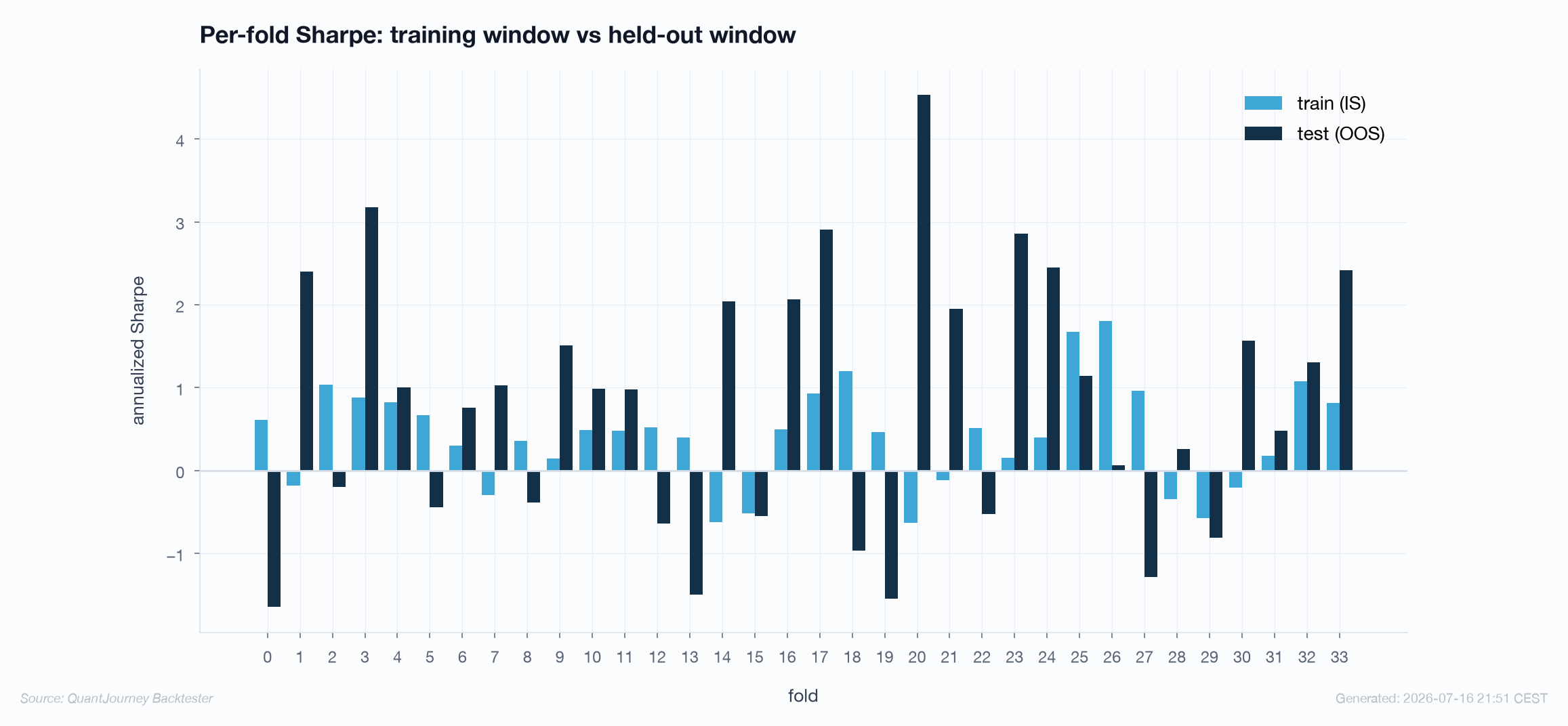
Before reading any aggregate, absorb the dispersion. A six-month window contains ~126 daily observations, so a under an IID approximation the annualized fold Sharpe has a one-standard-error uncertainty of roughly ±1.4. A two-sided 90% interval has a much wider half-width, about ±2.3, before accounting for autocorrelation and non-normality. Single-fold numbers around ±2 are therefore unsurprising:
This is why the composite matters and individual folds mostly do not: stitching the 34 test windows into one 17-year OOS return path pools the noise down. The stitched path is the dark line below — and its verdict for this strategy is an OOS Sharpe of 0.513, CAGR 5.14%, max drawdown −22.2%, with a bootstrap 90% CI on the Sharpe of [0.16, 0.90]. Positive, modest, uncertain — exactly what a plain trend rule on liquid ETFs should honestly look like.
The full result object is a first-class audit trail, not a scalar:
result.mode              # "slice_diagnostics" | "per_fold_refit"
result.n_folds           # 34
result.oos_sharpe        # 0.513   <- the composite stitched-OOS number
result.oos_cagr          # 0.0514
result.oos_max_dd        # -0.222
result.overfit_ratio     # 0.51    IS Sharpe / OOS Sharpe
result.efficiency        # 2.13    OOS CAGR / IS CAGR
result.sharpe_decay      # +0.012  slope of OOS Sharpe across folds
result.sharpe_ci_5pct    # 0.16    stationary-bootstrap CI on the OOS path
result.sharpe_ci_95pct   # 0.90
result.deflated_sharpe   # or None + result.deflated_sharpe_reason
result.deflated_sharpe_method  # pooled WF DSR-style | PSR N=1 | None
result.walk_forward_top_k_rank_failure_rate  # or None
result.rank_stability_reason                  # explains unavailability

for fr in result.folds:  # per-fold audit trail
    fr.fold.train_start, fr.fold.oos_start, fr.is_sharpe, fr.oos_sharpe
Overfit ratio, efficiency, decay — and their traffic lights
Three summary ratios compress the IS/OOS relationship. They are conventions with thresholds, not laws — the engine labels them as such.
| Metric | Green | Yellow | Red | This run |
|---|---|---|---|---|
| Overfit ratio (IS/OOS Sharpe) | < 1.5 | 1.5 – 2.5 | > 2.5 — likely overfit | 0.51 |
| Efficiency (OOS/IS CAGR) | > 0.7 | 0.4 – 0.7 | < 0.4 — poor transfer | 2.13 |
| Sharpe decay (slope across folds) | > −0.01 | −0.01 – −0.05 | < −0.05 — alpha decaying | +0.012 |
Note the direction of this run's "anomalies": OOS beat IS (ratio 0.51, efficiency above 2). No magic — no parameter fitting occurs inside this example, so optimizer overfit is not the explanation; external rule, universe and fold selection can still overfit. The rolling training windows keep containing 2008, 2015 and 2022 while several test windows landed in recoveries. Ratios below 1 are a property of the sample, not a virtue of the strategy; ratios far above the thresholds are the actionable warning. The engine ships the thresholds as code, with context gates so a tiny fold count or a losing composite never renders green:
from backtester.walkforward.statistics.interpretation import interpret_metrics

verdicts = interpret_metrics({
    "overfit_ratio": result.overfit_ratio,
    "efficiency": result.efficiency,
    "sharpe_decay": result.sharpe_decay,
    "composite_sharpe": result.oos_sharpe,   # context: gates the lights
    "n_folds": result.n_folds,               # so tiny samples never show green
})
for v in verdicts:
    print(v)   # traffic-light verdict + the convention behind it
What the engine refuses to tell you
Two statistics in the result exist precisely to catch selection bias — and on this run the engine reports them as unavailable, with reasons, because they would be meaningless.
# The engine refuses to fake statistics it cannot honestly compute.
# From the run on this page (fixed parameters, no optimizer):

result.deflated_sharpe        # None
result.deflated_sharpe_reason
# "in-sample; DSR not meaningful without independent trials"

result.walk_forward_top_k_rank_failure_rate   # None
result.rank_stability_reason
# "requires per-trial OOS evaluation; set WalkForwardConfig.rank_stability_trials=K
#  (>=2) with an optimizer to evaluate top-K trials OOS per fold"

# A number that cannot be computed is reported as unavailable WITH the
# reason - never silently as zero. (ADR-431 discipline.)
In this page's slice-diagnostics mode, the purported OOS series is still cut from one in-sample
run, so a Sharpe-selection probability is unavailable regardless of whether an optimizer exists. In a causal
per-fold run with no optimizer population, the calculation reduces to PSR with effective N = 1 and is labelled
probabilistic_sharpe_n1. With nested optimization, pooled objectives from different training folds
produce an explicitly labelled pooled_walk_forward_dsr_style diagnostic — useful, but not canonical
DSR for one common trial population. The
walk-forward top-K rank failure rate measures how often the IS winner falls below the midpoint
of the top-K subset on rolling OOS folds. It is not canonical CSCV PBO. Without per-trial OOS evaluations there
are no ranks. The rolling rank diagnostic becomes available when a search runs inside the walk-forward (set
rank_stability_trials=K and pass an optimizer= — the
Optuna guide does exactly that). A tool that printed 0.0 instead of
"unavailable + reason" would fabricate reassurance.
Run it
Both modes ship as runnable examples; the environment switch makes the evidence class explicit in the command itself.
# Slice diagnostics over one full-period run (fast)
./strategy.sh example_wf_01_rolling_walkforward

# Separate date-bounded execution for every fold (the OOS claim)
QJ_WF_MODE=per_fold_refit ./strategy.sh example_wf_01_rolling_walkforward

# Anchored scheme with a larger pre-OOS purge
QJ_WF_MODE=per_fold_refit ./strategy.sh example_wf_03_anchored_purge_embargo
Before calling a result out of sample
Freeze the research decision first
Universe, features, objective, parameter bounds, costs and fold geometry are fixed before any test window is read.
Fit inside training only
Every learned quantity — parameters, scalers, pair choices, covariances — uses the fold's training observations, then stays frozen through its test window.
Use per-fold refit for the claim
Slice diagnostics inform; date-bounded fold execution is what supports the words "out of sample". Label which one you ran.
Read the dispersion before the composite
12/34 negative folds is normal for a real edge. One dominant fold is the red flag — check concentration before averaging it away.
Never revise mid-walk
Changing the strategy after seeing fold 20 and reporting folds 21–34 as pristine converts the whole exercise into in-sample fiction.
Archive fold-level artifacts
Dates, per-fold metrics, the config and its seed — the composite is a claim; the folds are the evidence.
We do independent validation engagements — permutation tests, walk-forward, Sharpe selection diagnostics and rank stability on your code or track record, delivered as a signed, reproducible report.
References
- Bailey, D. H., Borwein, J., López de Prado, M. & Zhu, Q. J. (2017). The Probability of Backtest Overfitting. Journal of Computational Finance 20(4) — CSCV and rank-based PBO.
- López de Prado, M. (2018). Advances in Financial Machine Learning, ch. 7 & 12 — purged k-fold, embargo and combinatorial purged CV.
- Pardo, R. (2008). The Evaluation and Optimization of Trading Strategies. Wiley — the original walk-forward analysis treatment.
- Lo, A. W. (2002). The Statistics of Sharpe Ratios. Financial Analysts Journal 58(4) — the standard error behind the fold-noise arithmetic.
- Politis, D. N. & Romano, J. P. (1994). The Stationary Bootstrap. JASA 89(428) — the resampling scheme behind the OOS Sharpe confidence interval.